A quick and easy multilayer model for Keras
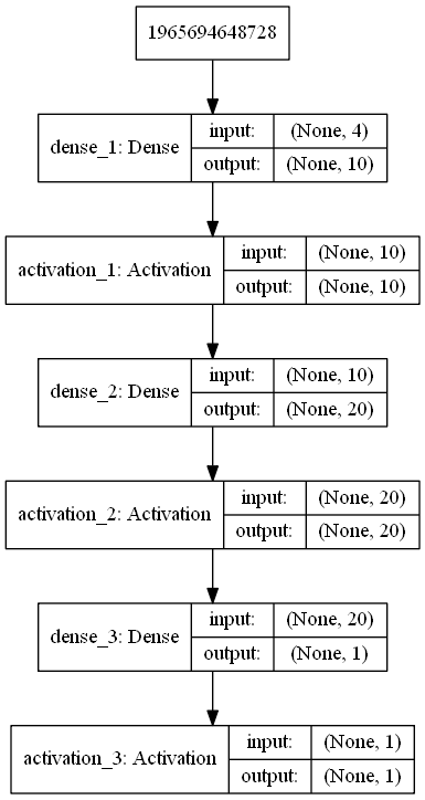
Hi there! today we will build a multilayer model that should be like this: ! .
.
The multilayer perceptron model will be fed with input data of shape 3 rows and 4 columns. Then we will evaluate or predict the model by giving an input to it. This process is quite simple but that is very important before moving towards complex data handling. Lets import the essential items
from keras.models import Sequential
from keras.layers import Dense, Activation
from keras.utils import plot_model
from keras.layers import Dense, Dropout
from keras.optimizers import SGD
We also need numpy library to stack vertically the data. Lets import numpy as np.
import numpy as np
Its time to build the model. The input of each sample fed to this model consists of 4 elements. So the input_shape will be (4,). It is used for single dimension. To make things very simple and easy to understand, I have made three samples i.e. [1,1,1,1], [2,2,2,2], and [3,3,3,3]. The output for each of them respectively is 1,2,3. It means that the model will take a sample [1,1,1,1] and it should output a value nearly or equal to 1, because our target is 1. Similarly for the input [2,2,2,2] the output should be nearly or equal to 2. Lets plot the model to have a look and compile it using SGD and our loss function is mean squared error. The metrics to monitor the performance of training process is accuracy.
model = Sequential()
model.add(Dense(10, input_shape=(4,)))
model.add(Activation('relu'))
model.add(Dense(20))
model.add(Activation('relu'))
model.add(Dense(1))
model.add(Activation('relu'))

plot_model(model, to_file='mymodel.png', show_shapes=True)
model.compile(loss='mean_squared_error',optimizer='sgd',metrics=['accuracy'])
As said earlier lets create the input data.
sample1 = np.array([1,1,1,1])
sample2 = np.array([2,2,2,2])
sample3 = np.array([3,3,3,3])
To feed this data lets stack them vertically.
data = np.vstack((sample1,sample2,sample3))
Now we need to define the target data in a similar way for the input data.
label1 = np.array([1])
label2 = np.array([2])
label3 = np.array([3])
labels = np.vstack((label1,label2,label3))
Its time to train the model using fit function. The number of epochs is set to 10, batch size is 3 which means 3 samples will be fed per epoch.
model.fit(data, labels, epochs=10, batch_size=3)
Alright so far so good. Lets predict the trained model using .predict function on the same input data.
out = model.predict(data)
print("Target is:", labels)
print("Prediction is:", out)
Here is the output of the full code of lab3.
3/3 [==============================] - 1s 463ms/step - loss: 0.4051 - acc: 0.3333
Epoch 2/10
3/3 [==============================] - 0s 997us/step - loss: 0.0115 - acc: 1.0000
Epoch 3/10
3/3 [==============================] - 0s 665us/step - loss: 7.3647e-04 - acc: 1.0000
Epoch 4/10
3/3 [==============================] - 0s 665us/step - loss: 1.0322e-04 - acc: 1.0000
Epoch 5/10
3/3 [==============================] - 0s 665us/step - loss: 7.0871e-05 - acc: 1.0000
Epoch 6/10
3/3 [==============================] - 0s 666us/step - loss: 6.8368e-05 - acc: 1.0000
Epoch 7/10
3/3 [==============================] - 0s 663us/step - loss: 6.7425e-05 - acc: 1.0000
Epoch 8/10
3/3 [==============================] - 0s 332us/step - loss: 6.6573e-05 - acc: 1.0000
Epoch 9/10
3/3 [==============================] - 0s 332us/step - loss: 6.5735e-05 - acc: 1.0000
Epoch 10/10
3/3 [==============================] - 0s 665us/step - loss: 6.4906e-05 - acc: 1.0000
Target is: [[1]
 [2]
 [3]]
Prediction is: [[1.0120525]
 [2.002926 ]
 [2.9938   ]]
Prediction is closer to the target. The accuracy has reached 1 and the mean_squared_error 6.4906e-05 is also good. Thats all for this lab 3. In the next lab 4 we will learn about training regression model and analyse the effect of number of Epochs on different performace meterics. I hope this lab will be helpful for the beginners. Code of lab is available.
