Learn SQL in a Single Post: Complete Tutorial From SELECT to Window Functions and ACID Transactions

SQL is the lingua franca of data. Whether you are building a backend API, analyzing product metrics, or running a data pipeline, SQL is the one language that touches every relational database on earth — Postgres, MySQL, SQLite, SQL Server, Oracle, even distributed engines like Snowflake and BigQuery. This single post teaches the whole language in five stages, with runnable snippets and five diagrams.

Learning Roadmap

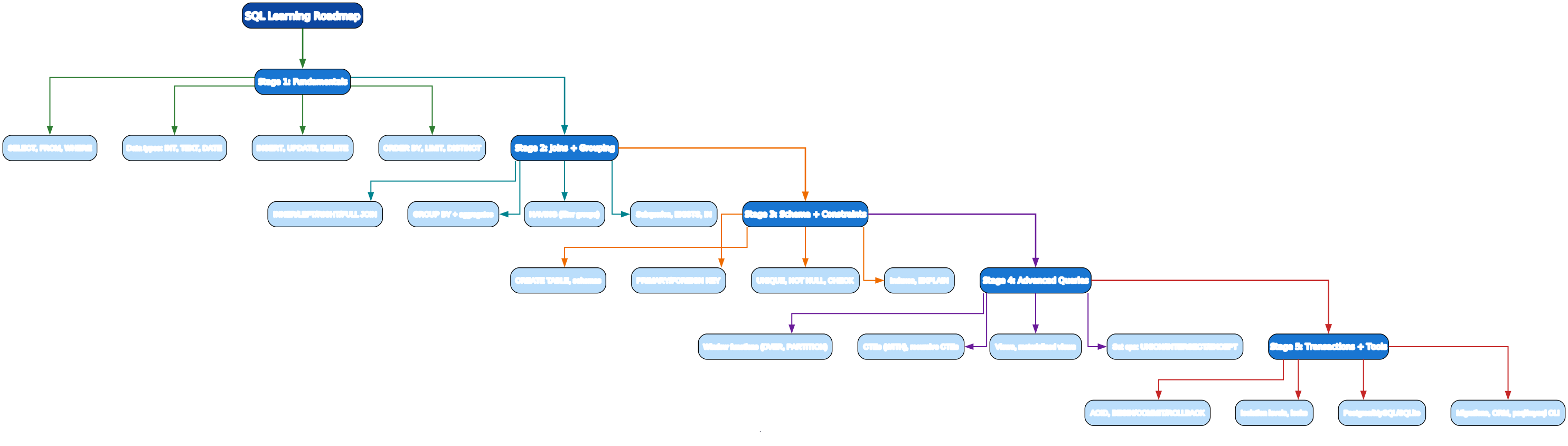
The roadmap moves from querying existing data (Stage 1), through combining and aggregating it (Stage 2), to defining your own schema (Stage 3), then advanced analytical SQL (Stage 4), and finally keeping data safe with transactions (Stage 5). Let us go stage by stage.

---

Stage 1 — Fundamentals: SELECT, Data Types, CRUD

The SELECT statement

Everything in SQL starts with SELECT:

-- pick columns from a table, filter, sort, limit
SELECT id, name, email
FROM users
WHERE active = TRUE
ORDER BY created_at DESC
LIMIT 10;

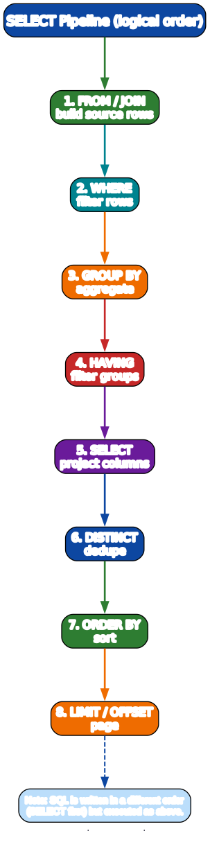
Logical execution order matters — SQL is written SELECT ... FROM ... WHERE ... but executed FROM → WHERE → GROUP BY → HAVING → SELECT → ORDER BY → LIMIT. Knowing this order prevents the classic bug of using a column alias in WHERE (it does not exist yet at that stage).

Core data types

Category	Types	Notes
Numeric	INT, BIGINT, DECIMAL(p,s), REAL, SERIAL	SERIAL auto-increments (Postgres); use DECIMAL for money
Text	VARCHAR(n), TEXT, CHAR(n)	TEXT is unbounded; VARCHAR(n) caps length
Time	DATE, TIME, TIMESTAMP, INTERVAL	TIMESTAMP WITH TIME ZONE for UTC-aware
Boolean	BOOLEAN	TRUE / FALSE / NULL
JSON	JSON, JSONB (Postgres)	JSONB is indexed binary JSON

CRUD: INSERT, UPDATE, DELETE

-- create
INSERT INTO users (name, email, active)
VALUES ('Ada Lovelace', 'ada@example.com', TRUE)
RETURNING id, created_at;                  -- Postgres returns the new row

-- update (ALWAYS include WHERE!)
UPDATE users
SET active = FALSE, updated_at = NOW()
WHERE last_login < NOW() - INTERVAL '1 year';

-- delete (ALWAYS include WHERE!!)
DELETE FROM users WHERE id = 42;

-- bulk insert
INSERT INTO products (name, price)
VALUES ('Widget', 9.99), ('Gadget', 14.99), ('Gizmo', 19.99);

Pitfall: An UPDATE or DELETE with no WHERE touches every row. Always run a SELECT with the same WHERE first to preview the affected rows.

Sorting, limiting, deduplication

SELECT DISTINCT country FROM users ORDER BY country;
-- pagination: page 3 of 10-per-page
SELECT * FROM products ORDER BY id ASC LIMIT 10 OFFSET 20;

---

Stage 2 — Joins + Grouping

Joins

Joins combine rows from two tables on a related column. This is the heart of relational SQL.

-- INNER JOIN: only users who placed an order
SELECT u.name, o.id AS order_id, o.total
FROM users u
INNER JOIN orders o ON u.id = o.user_id;

-- LEFT JOIN: ALL users, with their orders (nulls if no orders)
SELECT u.name, o.id AS order_id
FROM users u
LEFT JOIN orders o ON u.id = o.user_id;

-- RIGHT JOIN: ALL orders, with their user (nulls if user deleted)
SELECT u.name, o.id
FROM users u
RIGHT JOIN orders o ON u.id = o.user_id;

-- FULL OUTER JOIN: every user and every order, matched where possible
SELECT u.name, o.id
FROM users u
FULL OUTER JOIN orders o ON u.id = o.user_id;

-- CROSS JOIN: cartesian product (every user x every product) — rare, careful
SELECT u.name, p.name
FROM users u CROSS JOIN products p;

-- SELF JOIN: employees and their managers in the same table
SELECT e.name AS employee, m.name AS manager
FROM employees e
LEFT JOIN employees m ON e.manager_id = m.id;

If the join column has the same name in both tables, USING (id) is shorthand for ON a.id = b.id.

GROUP BY + aggregates

Aggregates collapse many rows into one: COUNT, SUM, AVG, MIN, MAX.

-- orders per user, with their total spend
SELECT u.id, u.name,
       COUNT(o.id)     AS order_count,
       COALESCE(SUM(o.total), 0) AS total_spend
FROM users u
LEFT JOIN orders o ON u.id = o.user_id
GROUP BY u.id, u.name
ORDER BY total_spend DESC;

COALESCE(x, 0) replaces NULL with 0 — essential because SUM over zero rows returns NULL, not 0.

HAVING — filtering groups

WHERE filters rows before grouping; HAVING filters groups after. This distinction trips up every SQL beginner:

-- only users with 3+ orders and total spend over $100
SELECT u.name, COUNT(o.id) AS n, SUM(o.total) AS spend
FROM users u JOIN orders o ON u.id = o.user_id
GROUP BY u.name
HAVING COUNT(o.id) >= 3 AND SUM(o.total) > 100;

Subqueries, IN, EXISTS

-- users who have never ordered (anti-join via NOT EXISTS)
SELECT u.* FROM users u
WHERE NOT EXISTS (SELECT 1 FROM orders o WHERE o.user_id = u.id);

-- products priced above the average
SELECT * FROM products
WHERE price > (SELECT AVG(price) FROM products);

-- orders from VIP users
SELECT * FROM orders
WHERE user_id IN (SELECT id FROM users WHERE tier = 'vip');

---

Stage 3 — Schema + Constraints + Indexes

CREATE TABLE

CREATE TABLE orders (
    id          BIGSERIAL    PRIMARY KEY,
    user_id     BIGINT       NOT NULL REFERENCES users(id) ON DELETE CASCADE,
    total       DECIMAL(10,2) NOT NULL CHECK (total >= 0),
    status      VARCHAR(20)  NOT NULL DEFAULT 'pending'
                 CHECK (status IN ('pending','paid','shipped','cancelled')),
    created_at  TIMESTAMPTZ  NOT NULL DEFAULT NOW()
);

-- add an index to speed up filtering by user_id
CREATE INDEX idx_orders_user_id ON orders(user_id);
-- composite index for common two-column filters
CREATE INDEX idx_orders_user_status ON orders(user_id, status);

Keys and constraints

Constraint	Purpose
PRIMARY KEY	Unique, non-null row identity (one per table)
FOREIGN KEY	Enforces referential integrity to another table
UNIQUE	No two rows share this column value
NOT NULL	Column cannot be NULL
CHECK (expr)	Row must satisfy the expression
DEFAULT x	Value used when not specified on insert

Indexes and EXPLAIN

Indexes are the single biggest performance lever. Without an index, WHERE user_id = 7 scans every row (sequential scan); with an index, it is a B-tree lookup.

-- see the query plan BEFORE running
EXPLAIN ANALYZE
SELECT * FROM orders WHERE user_id = 7 AND status = 'paid';

If EXPLAIN shows a Seq Scan on a large table where you filter a column, add an index on that column. If it shows an Index Scan or Index Only Scan, the index is working.

Pitfall: Indexes speed up reads but slow down writes (each INSERT/UPDATE must update the index). Do not index every column — index the ones in WHERE, JOIN ON, and ORDER BY.

---

Stage 4 — Advanced Queries: Window Functions, CTEs, Views

Window functions

Window functions compute a value across a set of rows related to the current row without collapsing rows (unlike GROUP BY). This is the single most powerful analytical SQL feature.

-- rank orders by total within each user, keep every row
SELECT u.name, o.id, o.total,
       ROW_NUMBER() OVER (PARTITION BY o.user_id ORDER BY o.total DESC) AS rn,
       RANK()       OVER (PARTITION BY o.user_id ORDER BY o.total DESC) AS rnk,
       SUM(o.total) OVER (PARTITION BY o.user_id)                       AS user_total,
       LAG(o.total) OVER (PARTITION BY o.user_id ORDER BY o.created_at) AS prev_total
FROM orders o JOIN users u ON u.id = o.user_id;

Common window functions:

• ROW_NUMBER() — unique sequential number within partition
• RANK() / DENSE_RANK() — rank with gaps / without gaps for ties
• LAG(x) / LEAD(x) — value from previous / next row
• SUM/AVG/MIN/MAX(x) OVER (...) — running or partitioned aggregate
• FIRST_VALUE(x) / LAST_VALUE(x) — first/last in frame

CTEs (WITH)

CTEs make complex queries readable by naming intermediate result sets:

WITH vip_users AS (
    SELECT id, name FROM users WHERE tier = 'vip'
),
vip_totals AS (
    SELECT vu.name, SUM(o.total) AS spend
    FROM vip_users vu JOIN orders o ON o.user_id = vu.id
    GROUP BY vu.name
)
SELECT * FROM vip_totals WHERE spend > 1000 ORDER BY spend DESC;

Recursive CTEs

Recursive CTEs walk graphs and trees — e.g. an org chart:

WITH RECURSIVE org_tree AS (
    -- anchor: top-level employees (no manager)
    SELECT id, name, manager_id, 1 AS depth
    FROM employees WHERE manager_id IS NULL
    UNION ALL
    -- recursive: employees whose manager is already in the tree
    SELECT e.id, e.name, e.manager_id, t.depth + 1
    FROM employees e JOIN org_tree t ON e.manager_id = t.id
)
SELECT name, depth FROM org_tree ORDER BY depth, name;

Views

A view is a saved query you can SELECT from like a table:

CREATE VIEW active_users AS
SELECT id, name, email FROM users WHERE active = TRUE;

SELECT * FROM active_users WHERE email LIKE '%@example.com';

-- materialized view caches the result (Postgres); refresh manually
CREATE MATERIALIZED VIEW order_stats AS
SELECT user_id, COUNT(*) AS n, SUM(total) AS spend FROM orders GROUP BY user_id;
REFRESH MATERIALIZED VIEW order_stats;

Set operations

-- emails in users UNION emails in subscribers (deduped)
SELECT email FROM users
UNION
SELECT email FROM subscribers;

-- UNION ALL keeps duplicates (faster)
SELECT email FROM users UNION ALL SELECT email FROM subscribers;

-- INTERSECT: in both; EXCEPT: in first but not second
SELECT email FROM users INTERSECT SELECT email FROM subscribers;
SELECT email FROM users EXCEPT    SELECT email FROM subscribers;

---

Stage 5 — Transactions + Toolchain

ACID and transactions

A transaction is a unit of work that is all-or-nothing — either every statement commits or none do. The ACID properties:

• Atomicity — all or nothing; a failure rolls back everything
• Consistency — the database moves from one valid state to another (constraints hold)
• Isolation — concurrent transactions don’t interfere (governed by isolation level)
• Durability — once committed, the change survives crashes

BEGIN;
  UPDATE accounts SET balance = balance - 100 WHERE id = 1;  -- debit
  UPDATE accounts SET balance = balance + 100 WHERE id = 2;  -- credit
  -- if anything fails here, both updates are undone
COMMIT;
-- or ROLLBACK; to abandon

Pitfall: Never leave a transaction open without COMMIT or ROLLBACK — it holds locks and blocks other transactions.

Isolation levels

Level	Prevents	Allows
READ UNCOMMITTED	—	dirty reads
READ COMMITTED (default, Postgres)	dirty reads	non-repeatable reads, phantoms
REPEATABLE READ	dirty + non-repeatable	phantoms (InnoDB MVCC prevents most)
SERIALIZABLE	all anomalies	lowest concurrency

SET TRANSACTION ISOLATION LEVEL SERIALIZABLE;
BEGIN; ...; COMMIT;

The toolchain

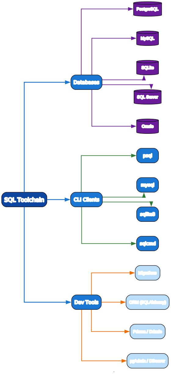
Databases:

• PostgreSQL — the gold-standard open-source RDBMS; richest feature set (JSONB, PARTITION, full-text, extensions like pgvector)
• MySQL — ubiquitous in web stacks (LAMP, WordPress); InnoDB engine
• SQLite — single-file, zero-config, embedded; perfect for apps, tests, and prototypes
• SQL Server / Oracle — enterprise commercial engines

CLI clients:

psql -h localhost -U postgres -d mydb     # Postgres
mysql -u root -p mydb                      # MySQL
sqlite3 app.db                             # SQLite

Migrations version-control your schema so every environment matches:

db/migrations/
  001_create_users.sql
  002_add_orders.sql
  003_add_index.sql

Tools: Flyway, golang-migrate, Alembic (Python), dbmate, Rails db:migrate.

ORMs map SQL to your language’s objects but should be understood as a convenience over SQL, not a replacement for it:

• Python: SQLAlchemy, Django ORM
• Node: Prisma, Drizzle
• Go: sqlx, GORM
• Rust: sqlx, Diesel, SeaORM

Pitfall: ORMs often generate N+1 queries (one query per row in a loop). Use EXPLAIN and eager-loading (selectinload, prefetch_related) to avoid it.

---

Quick-Start Checklist

1. Install a database. Postgres (docker run -e POSTGRES_PASSWORD=secret -p 5432:5432 postgres) or SQLite (sqlite3 test.db — zero install).
2. Connect with the CLI (psql / mysql / sqlite3) and run a SELECT.
3. Create a table with PRIMARY KEY, FOREIGN KEY, and sensible NOT NULL/CHECK constraints.
4. Write CRUD — INSERT, SELECT, UPDATE, DELETE — always with WHERE on updates/deletes.
5. Learn one join type a day — start with INNER, then LEFT, then the rest.
6. Aggregate with GROUP BY + HAVING and use COALESCE to handle NULLs.
7. Add indexes on filter/join columns and verify with EXPLAIN ANALYZE.
8. Master window functions (OVER, PARTITION BY, ROW_NUMBER, LAG) — they unlock analytics.
9. Wrap multi-step writes in transactions (BEGIN/COMMIT/ROLLBACK).
10. Set up migrations so your schema is reproducible.

Common Pitfalls

• UPDATE/DELETE without WHERE — affects every row. Always preview with SELECT first.
• Forgetting the logical execution order — you cannot use a SELECT alias in WHERE or GROUP BY (it does not exist yet); you can in ORDER BY and HAVING (some DBs).
• SUM/COUNT over no rows returns NULL/0 — use COALESCE(SUM(x), 0) to be safe.
• WHERE vs HAVING — WHERE filters rows before grouping, HAVING filters groups after.
• Missing indexes on foreign keys — joins and ON DELETE CASCADE get slow; index your FKs.
• Over-indexing — every index slows writes; index only what you filter/sort/join on.
• Leaving transactions open — holds locks; always COMMIT or ROLLBACK.
• N+1 queries from ORMs — eager-load relations.

Further Reading

• PostgreSQL Documentation — the most thorough free SQL reference
• SQL Tutorial (sqlzoo.net) — interactive exercises
• Use The Index, Luke! — the definitive guide to indexes
• PostgreSQL Tutorial — hands-on Postgres lessons
• Mode SQL Tutorial — analytics-focused, good on window functions

Related guides

Once you know SQL, these adjacent PyShine tutorials round out the backend and data stack:

• Build Your Own X: Master Programming by Recreating Technologies — includes building your own database from scratch to understand how SQL engines work.
• Learn Python in One Post: Complete Tutorial — pair SQL with Python via SQLAlchemy for the classic backend stack.
• Learn Go in One Post: Complete Tutorial — database/sql and connection pooling in Go.
• Learn Rust in One Post: Complete Tutorial — sqlx and type-safe SQL in Rust.

---

SQL rewards depth. Spend a week on each stage and you will move from “I can write a SELECT” to “I can design a schema, optimize a query plan, and reason about transaction isolation” — the skill set that separates a junior backend developer from a senior one. Run every snippet above against a real Postgres or SQLite database; reading SQL is no substitute for writing it.

Enjoyed this post? Never miss out on future posts by following us