Learn Computer Architecture in a Single Post: Complete Tutorial From CPU Pipeline to Memory Hierarchy, Cache, and Multicore

Computer architecture is the study of how a CPU works at the hardware level — how it fetches, decodes, executes, and writes back instructions, how it manages the memory hierarchy (registers → cache → RAM → disk), and how multiple cores coordinate. Understanding this is what lets you write code that runs fast — not just “the right algorithm” but “the right data layout” and “the right access pattern.” This single post covers the whole subject in five stages, with hand-drawn diagrams.

Learning Roadmap

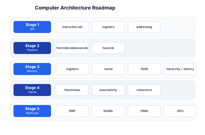
The roadmap moves from the instruction set (Stage 1), through the pipeline (Stage 2), the memory hierarchy (Stage 3), cache behavior (Stage 4), and multicore architecture (Stage 5). The Operating Systems tutorial and Compilers tutorial are the companion pieces — this is the hardware layer underneath both.

---

Stage 1 — The ISA: Instruction Set, Registers, Addressing

The Instruction Set Architecture

The ISA (Instruction Set Architecture) is the contract between the hardware and the software — the set of instructions the CPU understands, the registers it has, and the addressing modes it supports. It’s the boundary the compiler targets and the CPU implements.

Registers

Register type	Example	What it holds
General purpose	RAX, R1	arithmetic, data, addresses
Program counter (PC)	RIP / PC	the address of the next instruction
Stack pointer (SP)	RSP	the top of the stack
Flags / status	RFLAGS	zero, carry, overflow, sign
Floating-point / vector	XMM0 (AVX)	SIMD / math data

A register access is 1 cycle — the fastest storage. The compiler’s biggest job is deciding which variables live in registers vs spill to RAM.

Addressing modes

How an instruction specifies its operands:

• Immediate: ADD R1, #5 — the value 5 is in the instruction
• Register: ADD R1, R2 — the value is in R2
• Direct/absolute: LOAD R1, [0x1000] — memory at address 0x1000
• Register indirect: LOAD R1, [R2] — memory at the address in R2
• Indexed: LOAD R1, [R2 + R3*8] — base + index × scale (array access)
• PC-relative: BRANCH +100 — jump 100 bytes ahead (position-independent code)

The compiler turns arr[i] into indexed addressing (R2 = base, R3 = i, scale = element size). Understanding addressing modes is how you understand why array traversal is fast (contiguous, predictable) and linked-list traversal is slow (pointer-chasing, cache-unfriendly).

RISC vs CISC

	RISC (ARM, RISC-V)	CISC (x86)
Instructions	simple, fixed length	complex, variable length
Memory access	load/store only (ALU only on registers)	some instructions operate on memory
Register count	many (32+)	fewer (16 GP on x86-64)
Pipelining	easy	complex (micro-op decoding)

Modern x86 decodes CISC instructions into RISC-like micro-ops internally, so the pipeline is effectively RISC behind the CISC facade.

---

Stage 2 — The CPU Pipeline

The 5-stage pipeline

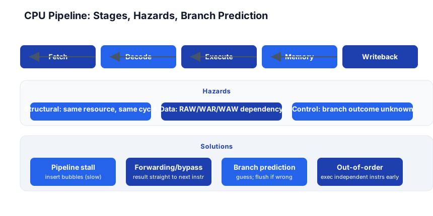
A CPU doesn’t execute one instruction at a time — it overlaps them in a pipeline, like a factory assembly line. Each stage handles one phase, and multiple instructions are in different stages simultaneously:

Cycle:    1       2       3       4       5
Instr 1:  Fetch → Decode → Execute → Mem → Writeback
Instr 2:          Fetch → Decode → Execute → Mem → Writeback
Instr 3:                  Fetch → Decode → Execute → Mem → Writeback

Stage	What it does
Fetch	get the instruction from memory (or L1i cache) at the PC
Decode	figure out what the instruction means (opcode + operands)
Execute	run the ALU operation (add, shift, compare)
Memory	read/write data memory (if load/store)
Writeback	write the result to the register file

With a 5-stage pipeline, 5 instructions can be in flight simultaneously — ideally, one instruction completes per cycle (IPC = 1).

Hazards — why the pipeline stalls

A hazard is a situation that prevents the next instruction from entering its stage on time:

• Structural hazard — two instructions need the same resource (e.g. one ALU). Fixed by stalling or adding resources.
• Data hazard (RAW) — instruction 2 needs the result of instruction 1, which hasn’t been written back yet. ADD R1, R2, R3 then SUB R4, R1, R5 — R1 isn’t ready.
• Control hazard — a branch instruction: the CPU doesn’t know which instruction comes next until the branch resolves (several cycles later). The pipeline stalls or guesses.

Solutions

• Pipeline stall (bubble) — insert a no-op cycle. Slow but correct.
• Forwarding / bypassing — route the ALU result directly to the next instruction, without waiting for writeback. Fixes most data hazards.
• Branch prediction — guess which way a branch goes (taken/not-taken). If right, no stall. If wrong, flush the pipeline (discard the speculative instructions) and restart from the correct path. Modern predictors are >95% accurate.
• Out-of-order execution — execute independent instructions out of program order (while preserving the appearance of in-order execution via a reorder buffer). This is why “instruction ordering” doesn’t strictly mean “the CPU does them top to bottom.”

Pitfall: Branch misprediction is expensive — flushing the pipeline wastes ~15-20 cycles on a deep pipeline. This is why predictable loops (for loops, simple ifs) are fast and unpredictable branches (data-dependent if/else, switch with random values) are slow. If you can eliminate a branch (bit manipulation, lookup table), you eliminate the misprediction penalty.

---

Stage 3 — Memory Hierarchy

The latency pyramid

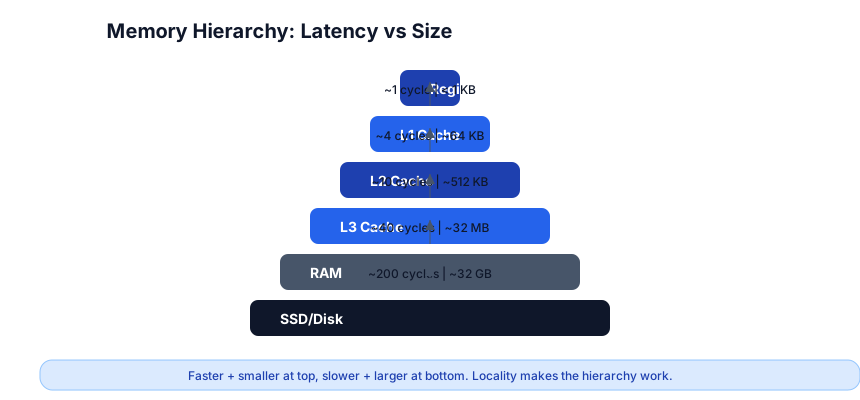
Level	Latency	Size	Notes
Registers	~1 cycle	< 1 KB	fastest; compiler manages
L1 Cache	~4 cycles	~64 KB	per-core, split D/I
L2 Cache	~10 cycles	~512 KB	per-core or shared
L3 Cache	~40 cycles	~32 MB	shared across cores
RAM	~200 cycles	~32 GB	main memory
SSD	~100k+ cycles	TB	non-volatile

The pyramid is 10^5× difference in speed from top to bottom — but also 10^9× difference in size. The reason it works: locality.

Temporal and spatial locality

• Temporal locality — if you accessed address A recently, you’ll probably access it again soon (the cache keeps it). Loops over the same data benefit.
• Spatial locality — if you accessed address A, you’ll probably access A+1, A+2, … soon (the cache fetches a cache line of ~64 bytes — the neighbors come free). Arrays benefit enormously; linked lists do not.

Why array traversal beats linked-list traversal

// Fast: contiguous memory, cache-friendly
for (int i = 0; i < n; i++) sum += arr[i];

// Slow: pointer-chasing, each node is a cache miss
for (Node* p = head; p; p = p->next) sum += p->val;

The array walks a contiguous block — the cache prefetcher sees the pattern and pre-fetches ahead. Each cache line (~64 bytes = 8 doubles) loads 8 elements at once. The linked list jumps to a random address for each node — every jump is a potential cache miss (~200 cycles vs ~4 cycles). This is why “the right algorithm” is necessary but not sufficient — the right data layout matters at the hardware level.

Pitfall: “Cache-friendly” isn’t about the algorithm — it’s about the memory access pattern. A sorting algorithm that touches a random array element per comparison (quicksort on a linked list) is slower than a “worse” algorithm that touches contiguous memory (insertion sort on an array) for small inputs, because the cache penalty dominates.

---

Stage 4 — Cache: Hits, Misses, Associativity, Coherence

Cache hits and misses

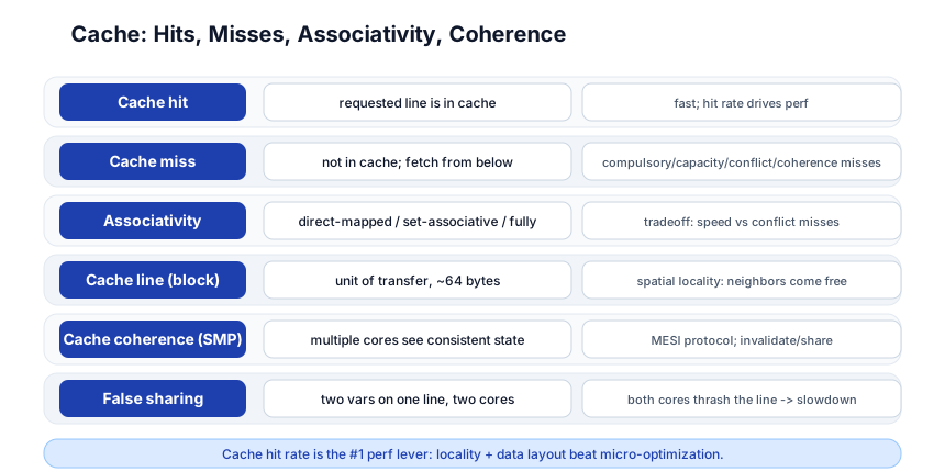
A cache hit — the requested data is in the cache (fast, ~4 cycles). A cache miss — it’s not, and the CPU fetches it from the next level (slow, ~200 cycles for a RAM miss). The hit rate is the fraction of accesses that hit; this is the single most important performance metric at the hardware level.

Cache misses categorized

• Compulsory (cold) miss — first access; the data was never in the cache. Unavoidable but limited (each line misses once).
• Capacity miss — the cache is too small to hold the working set; old data is evicted, then re-accessed.
• Conflict miss — multiple addresses map to the same cache set (in a direct-mapped cache), thrashing.
• Coherence miss — another core invalidated this cache line (in a multicore system).

Associativity

Type	What it means	Tradeoff
Direct-mapped	each address → 1 cache line slot	fast lookup, more conflict misses
Set-associative	each address → N possible slots (N-way)	fewer conflict misses, slightly slower
Fully associative	any address → any slot	fewest misses, slowest lookup

Most L1 caches are 8-way set-associative; L3 is 16-way or more.

Cache lines and false sharing

A cache line (typically 64 bytes) is the unit of transfer between cache and RAM — you can’t load a single byte; you load 64 bytes at a time. This is why contiguous arrays are fast (spatial locality) and scattered data is slow.

False sharing — two variables that happen to be on the same 64-byte cache line, accessed by different cores. Core A writes to variable X; Core B writes to variable Y (same line). Every write invalidates the other core’s copy (MESI protocol), causing both to thrash the line back and forth — a performance disaster even though the variables are logically independent.

Fix: pad the data so each variable is on its own cache line (align to 64 bytes). In C: _Alignas(64). In Go: padding fields. This is a real, measurable optimization for high-performance concurrent code.

Cache coherence (MESI)

In a multicore system, each core has its own L1/L2 cache. When core A modifies a cache line, core B’s copy is stale. The MESI protocol (Modified, Exclusive, Shared, Invalid) coordinates: a write invalidates other cores’ copies; the next read fetches the fresh version. This is how the hardware ensures the illusion of a single shared memory, even though caches are private per core.

Pitfall: False sharing is invisible in the source code — two unrelated variables on the same line, each accessed by a different thread, silently destroys performance. It’s a multicore bug that doesn’t crash but slows you down 10-100×. Always pad hot concurrent data to cache-line boundaries.

---

Stage 5 — Multicore: SMP, NUMA, SIMD, GPU

SMP vs NUMA

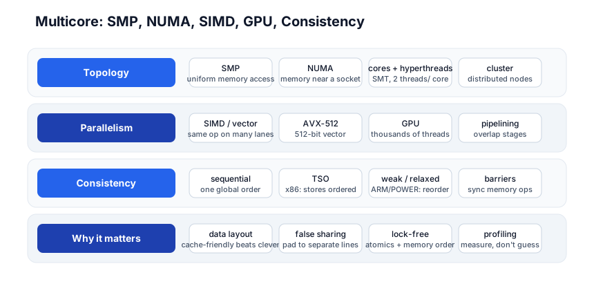
• SMP (Symmetric Multiprocessing) — all cores access the same RAM at the same speed (uniform memory access). Simple model; all cores are equal.
• NUMA (Non-Uniform Memory Access) — multi-socket systems where each CPU socket has “nearby” RAM (local) and “far” RAM (on another socket). Accessing local RAM is fast; accessing remote RAM is ~2× slower. The OS and the application need to be NUMA-aware (allocate memory on the node that will use it; schedule threads on the node near their data).

SIMD / vector instructions

SIMD (Single Instruction, Multiple Data) — one instruction operates on multiple data elements simultaneously. AVX-512 processes 16 floats or 8 doubles in one instruction. This is how matrix multiply, image processing, and crypto go fast — the compiler auto-vectorizes, or you use intrinsics/assembly.

GPU architecture

A GPU has thousands of simple cores, optimized for throughput (many parallel threads) rather than latency (one fast thread). It uses SIMT (Single Instruction, Multiple Threads) — groups of 32 threads execute the same instruction. GPUs are for massively parallel, data-parallel work (ML, rendering, simulation); they’re bad at branching (divergent threads within a warp serialize).

Memory consistency models

Model	What it guarantees	Example
Sequential consistency	all operations happen in program order, globally	the simplest to reason about, but slow
TSO (Total Store Order)	stores are ordered, but loads can pass stores	x86 (Intel, AMD)
Weak / relaxed	almost any reorder allowed; barriers needed	ARM, POWER, RISC-V

On x86 (TSO), stores are visible in order — x = 1; y = 2 is visible in that order to other cores. On ARM (weak), the store to y can be visible before x — you need a memory barrier (DMB on ARM) to force ordering. This is why lock-free code that works on x86 can break on ARM: x86 is more forgiving, ARM is not.

Pitfall: Writing lock-free code on x86 and assuming it’s correct, then deploying on ARM — the ARM weak memory model can reorder stores, and your “correct” x86 code races. Always use the right memory-ordering primitives (std::atomic with memory_order_* in C/C++, Ordering in Rust) — never rely on the hardware being “nice.”

---

Quick-Start Checklist

1. Learn the ISA basics — what registers, instructions, and addressing modes your platform has.
2. Understand the pipeline — fetch/decode/execute/writeback, and why hazards stall it.
3. Know the latency hierarchy — register (1ns) vs L1 (1ns) vs RAM (100ns) vs SSD (100µs). The gap is the key insight.
4. Think about locality — temporal (reuse) + spatial (contiguous) drive cache hit rate.
5. Prefer arrays over linked lists — contiguity is the #1 data-layout performance lever.
6. Avoid unpredictable branches — each misprediction flushes ~15 cycles. Use bit ops or lookup tables.
7. Align + pad hot data — false sharing (same cache line, different cores) is a silent 10-100× slowdown.
8. Know your memory model — x86 (TSO) is forgiving; ARM (weak) is not. Use proper atomics.
9. Profile with hardware counters — cache-miss rate, branch-mis prediction rate, not just wall-clock time.
10. Measure, don’t guess — perf stat, VTune, or ARM Streamline show cache miss rates and branch prediction rates.

Common Pitfalls

• Pointer-chasing (linked lists) — every node is a cache miss; use arrays.
• Unpredictable branches — each misprediction flushes the pipeline; prefer branchless code for random data.
• False sharing — two variables on one cache line, two cores, silent 10-100× slowdown.
• Assuming x86 memory model on ARM — x86 is TSO (ordered); ARM is weak (reorders stores). Use proper atomics.
• Iterating a column instead of a row — C is row-major; iterating column-jumped (A[0][0], A[1][0], …) thrashes the cache. Iterate rows first.
• Ignoring SIMD — the compiler can auto-vectorize loops, but only if the data is contiguous and the loop is simple. Help it.
• Optimizing without profiling — cache-miss rate and branch-misprediction rate tell you where the time actually goes. Measure first.

Further Reading

• Computer Architecture: A Quantitative Approach by Hennessy & Patterson — the canonical textbook
• Computer Systems: A Programmer’s Perspective by Bryant & O’Hallaron — the practical companion
• What Every Programmer Should Know About Memory by Ulrich Drepper — the definitive cache guide
• MIT 6.004 — free MIT architecture course
• perf Wiki — Linux hardware-performance profiling

Related guides

Computer architecture is the hardware layer under systems programming — these PyShine tutorials connect to it:

• Learn Operating Systems in One Post — virtual memory, context switches, and scheduling sit on this hardware.
• Learn Compilers in One Post — the compiler targets the ISA; instruction selection + register allocation.
• Learn C++ in One Post — C++ is the language closest to the hardware; alignas, std::atomic, SIMD intrinsics.
• Learn Rust in One Post — Ordering and atomics map directly to memory consistency models.
• Learn Data Structures and Algorithms in One Post — Big-O is the algorithm side; cache-friendly data layout is the architecture side. Both matter.

---

Computer architecture is the subject that separates “I can write code that runs” from “I can write code that runs fast.” The five stages here — ISA, pipeline, memory hierarchy, cache, multicore — cover the whole hardware stack, from a single instruction to a multi-socket NUMA system with SIMD and GPU offload. The two insights that pay off forever: the memory hierarchy is 10^5× difference in speed (locality + data layout beat micro-optimization), and the memory model matters across architectures (x86 is forgiving; ARM is not — use proper atomics). Learn the latency numbers, think about how your data is laid out in memory, and profile with hardware counters — once you’ve seen a cache-miss rate in the profiler, you’ll never write a linked list for hot data again.

Enjoyed this post? Never miss out on future posts by following us