Learn Data Structures and Algorithms in a Single Post: Complete Tutorial From Big-O to Dynamic Programming

Data structures and algorithms (DSA) is the grammar of computing. Every program stores data some way and processes it some way; DSA is the study of which ways are fast, which are slow, and why. It’s also the bedrock of technical interviews and the lens through which you read any codebase. This single post teaches the whole subject in five stages, with hand-drawn diagrams and runnable snippets.

Learning Roadmap

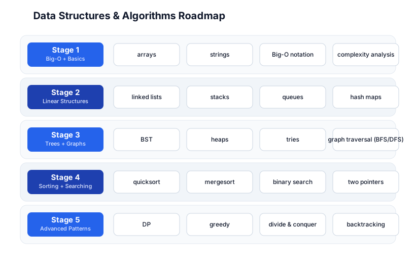
The roadmap moves from complexity analysis (Stage 1), through the linear data structures (Stage 2), to trees and graphs (Stage 3), the classic algorithms (Stage 4), and the advanced patterns that tie them together (Stage 5).

---

Stage 1 — Big-O + Basics

Big-O notation

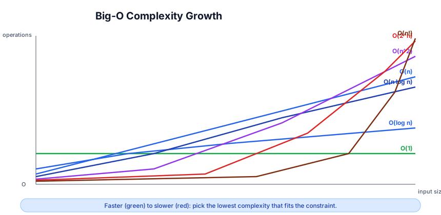
Big-O describes how an algorithm’s time or space grows as the input n grows — dropping constants and lower-order terms. It’s about scale, not exact speed.

Complexity	Name	Example
O(1)	constant	array index access
O(log n)	logarithmic	binary search
O(n)	linear	scan an array
O(n log n)	linearithmic	efficient sorts (quicksort, mergesort)
O(n²)	quadratic	nested loops, bubble sort
O(2ⁿ)	exponential	naive recursion (naive Fibonacci, N-queens)
O(n!)	factorial	all permutations

Pitfall: Big-O drops constants, so O(100n) is O(n). That’s why a “slower” O(n) algorithm can beat an O(n²) one on small inputs — the constant matters below a threshold. Big-O tells you what wins as n → ∞.

Arrays and strings

An array is a contiguous block of memory; indexing is O(1) because the address is computed directly. Inserting in the middle is O(n) because every later element shifts.

nums = [1, 2, 3, 4, 5]
nums[2]            # O(1) access
nums.append(6)     # amortized O(1)
nums.insert(0, 0)  # O(n) — shifts everything

A string is (conceptually) an array of characters — immutable in Python/Java, so s += "x" is O(n) (builds a new string). Use a list + "".join for repeated concatenation.

Complexity analysis rules

• A loop over n items: O(n).
• A nested loop over n × n: O(n²).
• A loop that halves the range each step (binary search): O(log n).
• A sort followed by a linear scan: O(n log n) + O(n) = O(n log n) (dominant term).
• Recursion: O(branching_factor ^ depth) if pure recursion; reduced by memoization.

---

Stage 2 — Linear Structures

Linked lists

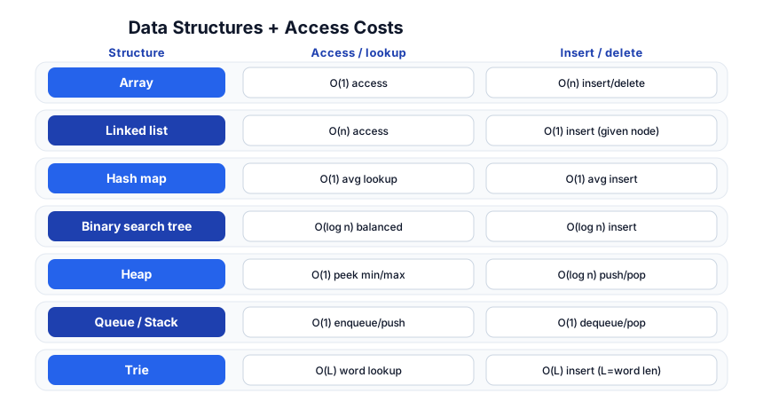
A linked list stores nodes with a value + a pointer to the next node. O(1) insert/delete given a node pointer, but O(n) access (you walk from the head).

class Node:
    def __init__(self, val, next=None):
        self.val, self.next = val, next

# singly linked list: 1 -> 2 -> 3
head = Node(1, Node(2, Node(3)))

# reverse it
def reverse(head):
    prev = None
    while head:
        nxt = head.next
        head.next = prev
        prev, head = head, nxt
    return prev

Pitfall: A classic interview trap — losing the rest of the list by reassigning head.next before saving head.next. Always save the next pointer first (as nxt above).

Stacks (LIFO)

A stack is last-in-first-out: push/pop are O(1). Use for undo, expression evaluation, balanced-parentheses, and DFS.

stack = []
stack.append(1); stack.append(2)
stack.pop()   # 2

Queues (FIFO)

A queue is first-in-first-out: enqueue/dequeue are O(1). Use for BFS, scheduling, buffering. In Python use collections.deque (O(1) on both ends); a plain list’s pop(0) is O(n).

from collections import deque
q = deque([1, 2, 3])
q.append(4); q.popleft()   # 1

Hash maps (dictionaries)

A hash map gives O(1) average lookup/insert/delete by hashing the key to a bucket. Worst case O(n) if all keys collide (rare with a good hash). This is the workhorse of “seen it before” problems (two-sum, frequency counts, caching).

seen = {}
for i, x in enumerate(nums):
    if target - x in seen:
        return [seen[target - x], i]
    seen[x] = i

Pitfall: Hash maps don’t preserve order (pre-3.7 Python, and in most languages). If you need order + O(1), use an ordered dict or a separate list.

Data structures + access costs

---

Stage 3 — Trees + Graphs

Binary search tree (BST)

A BST keeps ordered data: left subtree < node < right subtree. Search/insert/delete are O(log n) if balanced — O(n) if degenerate (like a linked list). Self-balancing variants (AVL, red-black) guarantee O(log n).

class TreeNode:
    def __init__(self, val, left=None, right=None):
        self.val, self.left, self.right = val, left, right

# in-order traversal of a BST yields sorted order
def inorder(node):
    if not node: return []
    return inorder(node.left) + [node.val] + inorder(node.right)

Heaps

A heap is a complete binary tree with the heap property (min-heap: parent ≤ children). The root is the min (or max). push/pop are O(log n); peek is O(1). Use for priority queues, top-K, and as the backbone of heapsort.

import heapq
h = []
heapq.heappush(h, 3); heapq.heappush(h, 1)
heapq.heappop(h)   # 1 (smallest)
# top-K largest: push into a min-heap of size K

Tries

A trie (prefix tree) stores strings by shared prefixes. Lookup/insert is O(L) where L is the word length — independent of how many words are stored. Used for autocomplete, dictionaries, IP routing.

Graphs

A graph is nodes (vertices) + edges. Represent as:

• Adjacency list — graph[u] = [v1, v2, ...] (sparse graphs; the default).
• Adjacency matrix — n × n matrix (dense graphs; O(1) edge lookup but O(n²) space).

# adjacency list
graph = {
    'A': ['B', 'C'],
    'B': ['D'],
    'C': ['D'],
    'D': [],
}

BFS — breadth-first search

Level by level, using a queue. Finds shortest path in an unweighted graph.

from collections import deque
def bfs(graph, start):
    visited, q, order = set(), deque([start]), []
    while q:
        node = q.popleft()
        if node in visited: continue
        visited.add(node); order.append(node)
        for n in graph[node]:
            if n not in visited: q.append(n)
    return order   # ['A','B','C','D']

DFS — depth-first search

Go deep first, using recursion (or an explicit stack). Used for connected components, topological sort, cycle detection.

def dfs(graph, node, visited=None):
    if visited is None: visited = set()
    visited.add(node)
    for n in graph[node]:
        if n not in visited: dfs(graph, n, visited)
    return visited

BFS vs DFS: BFS = shortest path (unweighted), level order; O(V+E). DFS = connectivity, topo sort, cycle detection; O(V+E). Both are O(V+E) with an adjacency list.

---

Stage 4 — Sorting + Searching

Sorting

Algorithm	Avg	Worst	Stable?	Notes
Quicksort	O(n log n)	O(n²)	no	in-place, fast in practice
Mergesort	O(n log n)	O(n log n)	yes	needs O(n) extra space
Heapsort	O(n log n)	O(n log n)	no	in-place
Counting sort	O(n + k)	O(n + k)	yes	when keys are small ints

Pitfall: sorted() in Python and Arrays.sort() in Java are O(n log n) and stable — just use them. Writing your own sort in an interview is rarely the point; knowing when each algorithm wins is.

Quicksort (the one to know)

def quicksort(a):
    if len(a) <= 1: return a
    pivot = a[len(a) // 2]
    left  = [x for x in a if x < pivot]
    mid   = [x for x in a if x == pivot]
    right = [x for x in a if x > pivot]
    return quicksort(left) + mid + quicksort(right)

Binary search

On a sorted array, binary search is O(log n). The bug-prone part is the boundary conditions.

def binary_search(a, target):
    lo, hi = 0, len(a) - 1
    while lo <= hi:
        mid = (lo + hi) // 2
        if a[mid] == target: return mid
        elif a[mid] < target: lo = mid + 1
        else: hi = mid - 1
    return -1

Pitfall: mid = (lo + hi) // 2 can overflow in languages with fixed ints (C/Java). Use mid = lo + (hi - lo) // 2. Python ints don’t overflow, but it’s the right habit.

Two pointers

A sorted-array pattern that turns O(n²) into O(n): one pointer at the start, one at the end, move them toward each other.

def two_sum_sorted(a, target):
    lo, hi = 0, len(a) - 1
    while lo < hi:
        s = a[lo] + a[hi]
        if s == target: return [lo, hi]
        elif s < target: lo += 1
        else: hi -= 1

Sliding window

For subarray/substring problems, a window [left, right] that expands and contracts — O(n) instead of O(n²).

def max_subarray_sum_k(a, k):
    window = sum(a[:k]); best = window
    for i in range(k, len(a)):
        window += a[i] - a[i - k]
        best = max(best, window)
    return best

---

Stage 5 — Advanced Patterns

Dynamic programming

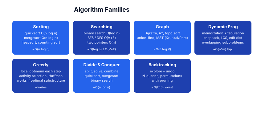
DP solves problems with overlapping subproblems and optimal substructure by caching subproblem results (memoization top-down, or tabulation bottom-up).

Fibonacci (the canonical example)

# naive recursion: O(2^n) — recomputes the same values
def fib_naive(n):
    return n if n < 2 else fib_naive(n-1) + fib_naive(n-2)

# memoization (top-down): O(n)
from functools import cache
@cache
def fib(n):
    return n if n < 2 else fib(n-1) + fib(n-2)

# tabulation (bottom-up): O(n), O(1) space
def fib(n):
    a, b = 0, 1
    for _ in range(n): a, b = b, a + b
    return a

0/1 Knapsack (the classic DP)

def knapsack(weights, values, capacity):
    dp = [0] * (capacity + 1)
    for w, v in zip(weights, values):
        for c in range(capacity, w - 1, -1):   # iterate backward for 0/1
            dp[c] = max(dp[c], dp[c - w] + v)
    return dp[capacity]

Pitfall: The 0/1 knapsack iterates c backward (so each item is used once); the unbounded knapsack iterates forward (items can repeat). Getting the direction wrong silently changes the answer.

Greedy

Greedy picks the locally optimal choice at each step. It works when the problem has the greedy-choice property (a local optimum is part of the global optimum) — e.g. activity selection, Huffman coding, Dijkstra. It fails when a locally bad choice would unlock a globally better one.

Divide and conquer

Split the problem, solve the halves, combine. Quicksort, mergesort, and binary search are all divide-and-conquer. The Master Theorem gives the complexity: T(n) = aT(n/b) + f(n).

Backtracking

Explore all possibilities by trying a choice, recursing, then undoing it. Used for permutations, combinations, N-queens, Sudoku. Pruning (skipping branches that can’t improve) is what makes it tractable.

def permutations(a):
    result = []
    def backtrack(path, remaining):
        if not remaining: result.append(path); return
        for i, x in enumerate(remaining):
            backtrack(path + [x], remaining[:i] + remaining[i+1:])
    backtrack([], a)
    return result

Interview prep

The patterns above cover the overwhelming majority of interview questions. The standard path:

• NeetCode 150 / Blind 75 — curated problem set that maps to these patterns.
• Practice one pattern at a time (not random problems) until you recognize the pattern from the problem statement.
• Always say the time/space complexity out loud before coding — that’s what interviewers grade.

---

The Toolchain

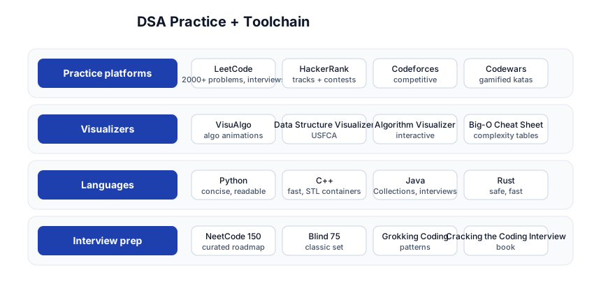
• Practice: LeetCode, HackerRank, Codeforces, Codewars.
• Visualizers: VisuAlgo, USFCA Data Structure Visualizer, Big-O Cheat Sheet.
• Languages: Python (concise, interview-friendly), C++ (fast, STL), Java, Rust.
• Interview prep: NeetCode 150, Blind 75, Cracking the Coding Interview.

---

Quick-Start Checklist

1. Learn Big-O cold — know O(1)/O(log n)/O(n)/O(n log n)/O(n²)/O(2ⁿ) and recognize them in code.
2. Master arrays + hash maps first — they solve most easy problems.
3. Learn the two-pointer and sliding-window patterns — they turn O(n²) into O(n) on sorted/contiguous data.
4. Know one sort (quicksort) and binary search — and their boundary bugs.
5. Learn BFS and DFS on graphs — they’re the same algorithm with a queue vs a stack.
6. Learn one tree (BST) and one heap — and when to use each.
7. Start DP with Fibonacci, then knapsack — memoization first, tabulation second.
8. Practice by pattern, not randomly — NeetCode 150 groups problems by pattern.
9. Always state time + space complexity before coding — it’s the interview grade.
10. Visualize on VisuAlgo when a data structure doesn’t click — seeing a heap push is worth a paragraph.

Common Pitfalls

• Off-by-one in binary search — lo <= hi vs lo < hi, and the +1/-1 on the bounds. Decide inclusive vs exclusive and stay consistent.
• Integer overflow in mid — use lo + (hi - lo) // 2 in C/Java.
• Modifying a list while iterating it — skip/delete bugs. Iterate over a copy, or use a separate result list.
• O(n) pop(0) on a Python list — use collections.deque.
• String concatenation in a loop — O(n²) for immutable strings; build a list and join.
• Forgetting to mark nodes visited in BFS/DFS — infinite loops on cyclic graphs.
• 0/1 vs unbounded knapsack direction — backward vs forward iteration.
• Greedy on a problem that needs DP — check for the greedy-choice property before reaching for greedy.
• Naive recursion without memoization — O(2ⁿ) when O(n) is a @cache away.

Further Reading

• Big-O Cheat Sheet — complexity reference
• VisuAlgo — algorithm visualizations
• NeetCode — curated roadmap + video solutions
• CP Algorithms — competitive-programming reference
• Introduction to Algorithms (CLRS) — the canonical textbook

Related guides

DSA underpins efficient code in every language — these PyShine tutorials apply it:

• Learn Python in One Post: Complete Tutorial — the snippets above are Python; pair DSA with Python’s collections (deque, Counter, heapq).
• Learn C++ in One Post: Complete Tutorial — STL containers (vector, unordered_map, priority_queue) are the interview-standard DSA toolkit.
• Learn Rust in One Post: Complete Tutorial — ownership makes linked structures harder; learn Rust’s Vec/HashMap/BinaryHeap approach.
• Learn SQL in One Post: Complete Tutorial — query planning is applied DSA (B-trees, hash joins, sort-merge).
• Learn Go in One Post: Complete Tutorial — Go’s built-in sort, container/heap, and maps are DSA in the standard library.

---

DSA is the subject where reading is no substitute for doing. The five stages here — Big-O, linear structures, trees and graphs, sorting and searching, advanced patterns — cover the whole map, but each only clicks once you’ve solved ten problems that use it. Spend a week per stage on NeetCode 150, state the complexity out loud every time, and within two months you’ll read a problem and know the pattern before you’ve finished the prompt. Run every snippet above; then go to LeetCode and solve the easy version of each pattern today.

Enjoyed this post? Never miss out on future posts by following us