Learn Deep Learning in a Single Post: Complete Tutorial From Neural Networks to Transformers and PyTorch Training

Deep learning is the branch of machine learning that uses neural networks — stacks of layers that learn hierarchical representations from data. It’s the technology behind image recognition, speech transcription, machine translation, and every large language model (GPT, Claude, Gemini). This single post teaches the whole field in five stages, with hand-drawn diagrams and runnable PyTorch.

Learning Roadmap

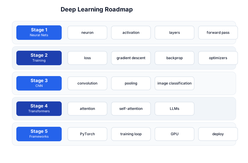
The roadmap moves from the neuron (Stage 1), through how it learns (Stage 2), the architectures for images and sequences (Stages 3-4), and the practical framework + deployment (Stage 5). The ML basics tutorial is the prerequisite — this post goes deep.

---

Stage 1 — Neural Networks

The neuron

A neuron is the unit of a neural network: it takes weighted inputs, sums them, adds a bias, and applies a non-linear activation function:

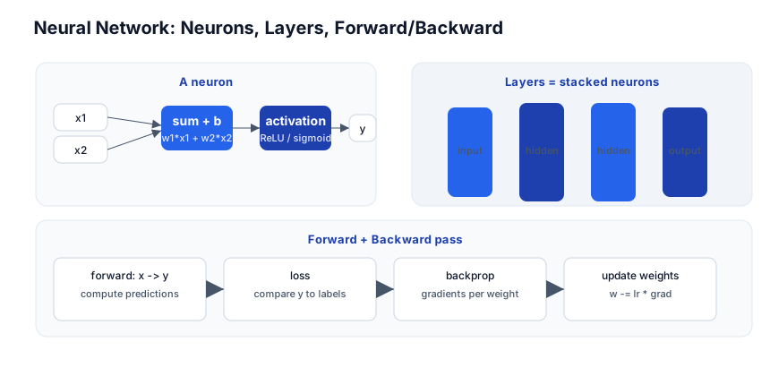
y = activation(w1*x1 + w2*x2 + ... + b)

• Weights (w1, w2, …) — learned parameters; they’re what the network learns.
• Bias (b) — a learned offset.
• Activation function — the non-linearity that lets the network learn complex patterns. Without it, a stack of linear layers is still linear (a composition of linear functions is linear).

Common activations

Function	Formula	Use
ReLU	max(0, x)	the default for hidden layers; simple, fast, no vanishing gradient for positive values
Sigmoid	1 / (1 + e^-x)	squashes to (0,1); binary classification output; vanishing gradient problem in deep nets
Tanh	(e^x - e^-x) / (e^x + e^-x)	squashes to (-1,1); similar vanishing issue
GELU	x * Phi(x)	used in transformers (smoother than ReLU)
Softmax	e^xi / sum(e^xj)	multi-class output (probabilities summing to 1)

Layers = stacked neurons

A layer is a set of neurons that all receive the same input and produce outputs that feed the next layer. A network is a stack of layers: input → hidden → hidden → … → output. The “deep” in deep learning = many layers, each learning progressively more abstract features.

import torch.nn as nn

model = nn.Sequential(
    nn.Linear(784, 128),   # input (28x28 pixels) -> 128 neurons
    nn.ReLU(),             # activation
    nn.Linear(128, 64),    # 128 -> 64
    nn.ReLU(),
    nn.Linear(64, 10),     # 64 -> 10 classes
)

The forward pass

The forward pass pushes input through the layers to get a prediction: y = model(x). Each layer transforms its input; the output of one layer is the input of the next.

---

Stage 2 — Training

The training loop

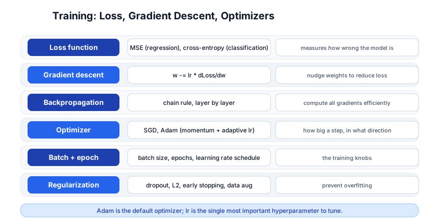
Training is a loop, repeated many times (epochs) over the dataset:

1. Forward pass — predictions = model(inputs)
2. Loss — compare predictions to true labels: loss = loss_fn(predictions, labels)
3. Backpropagation — compute the gradient of the loss w.r.t. every weight: loss.backward()
4. Update — nudge weights to reduce loss: optimizer.step()

import torch
import torch.nn as nn
import torch.optim as optim

model = nn.Sequential(nn.Linear(784, 128), nn.ReLU(), nn.Linear(128, 10))
loss_fn = nn.CrossEntropyLoss()
optimizer = optim.Adam(model.parameters(), lr=1e-3)

for epoch in range(10):
    for X_batch, y_batch in dataloader:
        pred = model(X_batch)              # forward
        loss = loss_fn(pred, y_batch)      # loss
        optimizer.zero_grad()
        loss.backward()                    # backprop (gradients)
        optimizer.step()                   # update weights
    print(f"epoch {epoch}, loss {loss.item():.4f}")

Loss functions

Loss	When
MSE (mean squared error)	regression (predict a number)
Cross-entropy	classification (predict a class)
Binary cross-entropy	binary classification
CTC	sequence-to-sequence with alignment (speech)

Gradient descent + optimizers

Gradient descent: w -= lr * gradient — step in the direction that reduces loss. The learning rate (lr) is the step size — too big and you overshoot/diverge; too small and you crawl. The optimizer decides how to step:

Optimizer	How
SGD	vanilla w -= lr * grad
SGD + momentum	add a running average of past gradients (smoother, faster)
Adam	adaptive per-parameter learning rate + momentum — the default
AdamW	Adam + decoupled weight decay (L2 regularization) — the modern default

Backpropagation

Backpropagation is the algorithm that computes all gradients efficiently using the chain rule: starting from the loss, it walks backward through the network, computing the derivative of the loss with respect to each weight layer by layer. PyTorch’s autograd does this automatically — you call loss.backward() and every weight’s .grad is populated.

Regularization — preventing overfitting

Technique	How
Dropout	randomly zero out neurons during training (forces redundancy)
L2 regularization (weight decay)	add lambda * sum(w^2) to the loss (penalize large weights)
Early stopping	stop when validation loss starts rising
Data augmentation	transform training data (flip, crop, rotate) to effectively get more
Batch normalization	normalize layer inputs per-batch (stabilizes training)

Pitfall: The learning rate is the single most important hyperparameter. Too high → the loss diverges (NaN). Too low → training takes forever. Start with 1e-3 for Adam, and use a learning rate schedule (warmup + decay) for large models. Always watch the training + validation loss curves.

---

Stage 3 — CNNs (Convolutional Neural Networks)

Why CNNs for images

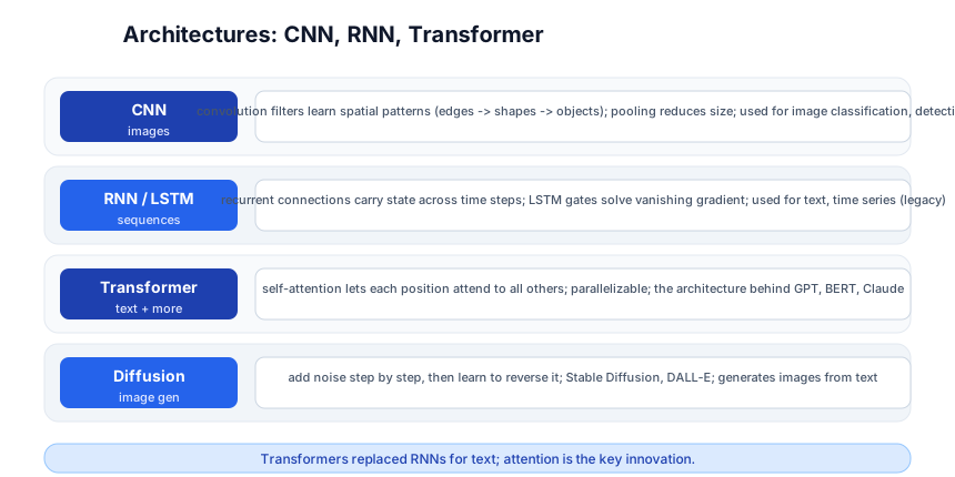
A fully-connected layer on an image would need millions of weights (every pixel to every neuron). A CNN uses convolutional filters — small learned kernels (e.g. 3x3) that slide across the image, detecting local patterns with far fewer parameters. Early layers detect edges; later layers detect shapes, then objects.

Convolution, pooling, and a typical architecture

import torch.nn as nn

cnn = nn.Sequential(
    nn.Conv2d(3, 32, 3, padding=1),    # 3 channels -> 32 filters, 3x3
    nn.ReLU(),
    nn.MaxPool2d(2),                    # downsample by 2
    nn.Conv2d(32, 64, 3, padding=1),
    nn.ReLU(),
    nn.MaxPool2d(2),
    nn.Flatten(),
    nn.Linear(64 * 8 * 8, 10),           # fully-connected -> 10 classes
)

• Conv2d — convolution: in_channels → out_channels filters.
• MaxPool2d — downsampling (take the max in each window); reduces spatial size, adds invariance.
• Flatten + Linear — convert the feature maps to a vector, then classify.

Famous CNN architectures

Architecture	Innovation
LeNet (1998)	the first CNN (handwritten digit recognition)
AlexNet (2012)	deep CNN + ReLU + GPU; started the deep learning era
ResNet (2015)	residual connections (skip connections) that enable very deep networks (50-152 layers)
EfficientNet	scaled width/depth/resolution together
Vision Transformer (ViT)	transformers applied to image patches (the modern alternative)

---

Stage 4 — Transformers

The problem with RNNs

RNNs (recurrent neural networks) process sequences one step at a time, carrying hidden state — but they’re sequential (can’t parallelize) and suffer from vanishing gradients on long sequences. LSTMs added gates to fix the gradient issue, but not the sequentiality.

The Transformer: self-attention

The Transformer (2017, “Attention Is All You Need”) replaced recurrence with self-attention: each position in the sequence attends to (weighs) all other positions simultaneously. This is parallelizable (process all positions at once on a GPU) and captures long-range dependencies far better.

Self-attention in one line: for each token, compute a weighted average of all tokens, where the weights are learned from the query-key dot product:

Attention(Q, K, V) = softmax(Q @ K^T / sqrt(d)) @ V

• Q (query) — “what am I looking for?”
• K (key) — “what do I contain?”
• V (value) — “what information do I carry?”
• softmax(Q @ K^T) — how much each position should attend to each other
• Multi-head attention — run multiple attention heads in parallel, each learning a different pattern

Transformers → LLMs

A large language model (GPT, Claude, Gemini) is a transformer trained on massive text:

• GPT-style (decoder-only): predicts the next token; autoregressive generation.
• BERT-style (encoder-only): bidirectional; used for understanding (classification, search).
• The model learns language, facts, and reasoning from the training data; fine-tuning + RLHF adapt its behavior.

Diffusion models

Diffusion (Stable Diffusion, DALL-E) generates images: add Gaussian noise to an image step by step, then train a neural network (often a U-Net) to reverse the process. At generation, start from pure noise and denoise into an image, conditioned on a text prompt (via a CLIP encoder).

Pitfall: Transformers are data-hungry — they need millions/billions of examples to train well. On small datasets, a CNN or a tree-based model (XGBoost) often wins. The “scale is all you need” approach only works with the data and compute to match.

---

Stage 5 — Frameworks, Training Loop, GPU, Deploy

PyTorch — the dominant framework

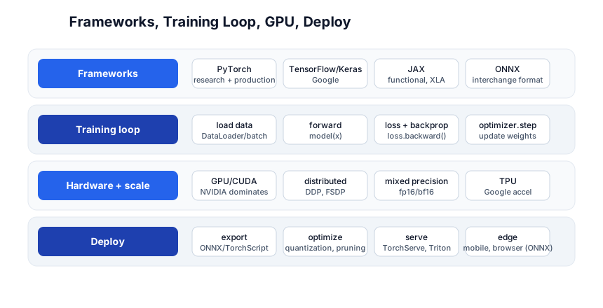
PyTorch is the default for research and increasingly production: eager execution (debuggable), dynamic graphs, a rich ecosystem (HuggingFace Transformers, torchvision, torchaudio). TensorFlow/Keras (Google) and JAX (functional, XLA-compiled) are alternatives.

# GPU
device = torch.device("cuda" if torch.cuda.is_available() else "cpu")
model = model.to(device)
X_batch, y_batch = X_batch.to(device), y_batch.to(device)

# mixed precision (2x faster, half the memory)
scaler = torch.amp.GradScaler()
with torch.amp.autocast():
    pred = model(X_batch)
    loss = loss_fn(pred, y_batch)
scaler.scale(loss).backward()
scaler.step(optimizer)
scaler.update()

The training loop (full)

for epoch in range(num_epochs):
    model.train()                          # training mode (dropout active)
    for X, y in train_loader:
        X, y = X.to(device), y.to(device)
        pred = model(X)
        loss = loss_fn(pred, y)
        optimizer.zero_grad()
        loss.backward()
        optimizer.step()
    
    model.eval()                           # eval mode (dropout off, batchnorm fixed)
    with torch.no_grad():                  # no gradients (saves memory)
        val_loss = sum(loss_fn(model(Xv), yv) for Xv, yv in val_loader)
    print(f"epoch {epoch}: train {loss:.4f} val {val_loss:.4f}")

Deploy

# export to ONNX (interchange format, runs on CPU/mobile/server)
torch.onnx.export(model, dummy_input, "model.onnx")
# or TorchScript for production serving
scripted = torch.jit.script(model)
scripted.save("model.pt")
# serve: TorchServe, NVIDIA Triton, or a FastAPI endpoint wrapping the model

---

Quick-Start Checklist

1. Install PyTorch (pip install torch torchvision); verify GPU with torch.cuda.is_available().
2. Write a 3-layer MLP on MNIST; train it for 5 epochs; watch the loss drop.
3. Learn the training loop: forward → loss → backward() → step().
4. Use Adam (lr=1e-3); if the loss diverges, lower the lr by 10x.
5. Watch train vs val loss — if val rises while train drops, you overfit (add dropout/early stop).
6. Build a CNN on CIFAR-10; see convolutions outperform the MLP.
7. Try a pretrained model — torchvision.models.resnet18(pretrained=True); fine-tune on your data.
8. Use HuggingFace Transformers — load a pretrained BERT/GPT in 3 lines.
9. Train on GPU with mixed precision; it’s 2-5x faster.
10. Export to ONNX and serve; or use a pre-trained model from HuggingFace Hub.

Common Pitfalls

• Learning rate too high — loss goes to NaN; reduce by 10x.
• Learning rate too low — loss barely moves; increase or use a schedule.
• Overfitting — train loss down, val loss up; add dropout, data augmentation, early stopping.
• Not setting model.train() / model.eval() — dropout and batchnorm behave differently; forgetting eval() gives wrong validation results.
• Forgetting optimizer.zero_grad() — gradients accumulate across batches; stale gradients corrupt training.
• Not using torch.no_grad() in evaluation — wastes memory computing gradients you don’t need.
• Data on CPU, model on GPU — every batch transfer is a bottleneck; move data to GPU once.
• Small data + big model — a transformer on 1,000 examples overfits instantly; use a pretrained model + fine-tune, or a simpler architecture.
• Not normalizing inputs — unnormalized data (pixels 0-255 instead of 0-1) makes training unstable.

Further Reading

• PyTorch Tutorials — the official starting point
• Deep Learning Book by Goodfellow et al — the theory reference (free)
• Dive into Deep Learning — interactive, PyTorch + theory
• HuggingFace Course — transformers + NLP
• Papers With Code — state of the art + implementations
• Andrej Karpathy’s YouTube — “Let’s build GPT” from scratch

Related guides

Deep learning builds on programming + math fundamentals — these PyShine tutorials connect to it:

• Learn Machine Learning in One Post — the prerequisite; ML basics before going deep.
• Learn Python in One Post — the language every DL framework uses; NumPy tensors are Python.
• Learn Data Structures and Algorithms in One Post — Big-O for model complexity; matrix math fundamentals.
• Learn PostgreSQL in One Post — pgvector stores and searches DL embeddings.
• Learn Docker in One Post — containerize model training and serving.

---

Deep learning’s power is the same idea repeated at scale: a layer learns a representation, the next layer builds on it, and a deep stack learns hierarchical features no human designed. The five stages here — neural networks, training, CNNs, transformers, frameworks — cover everything from a single neuron to a billion-parameter LLM. The two habits that pay off: start with a pretrained model and fine-tune (don’t train from scratch unless you have the data), and watch the training + validation loss curves — they tell you everything about what’s happening. Install PyTorch, train a 3-layer net on MNIST for 5 epochs, and watch the loss drop — that’s the moment it clicks.

Enjoyed this post? Never miss out on future posts by following us