Learn Machine Learning in a Single Post: Complete Tutorial From Supervised Learning to Neural Networks and the ML Workflow

Machine learning is the practice of building systems that learn patterns from data instead of being explicitly programmed. It powers search ranking, recommendation, fraud detection, speech recognition, self-driving perception, and every modern AI product. This single post teaches the whole field in five stages, with hand-drawn diagrams and runnable Python snippets — from the simplest linear model to what a neural network actually does.

Learning Roadmap

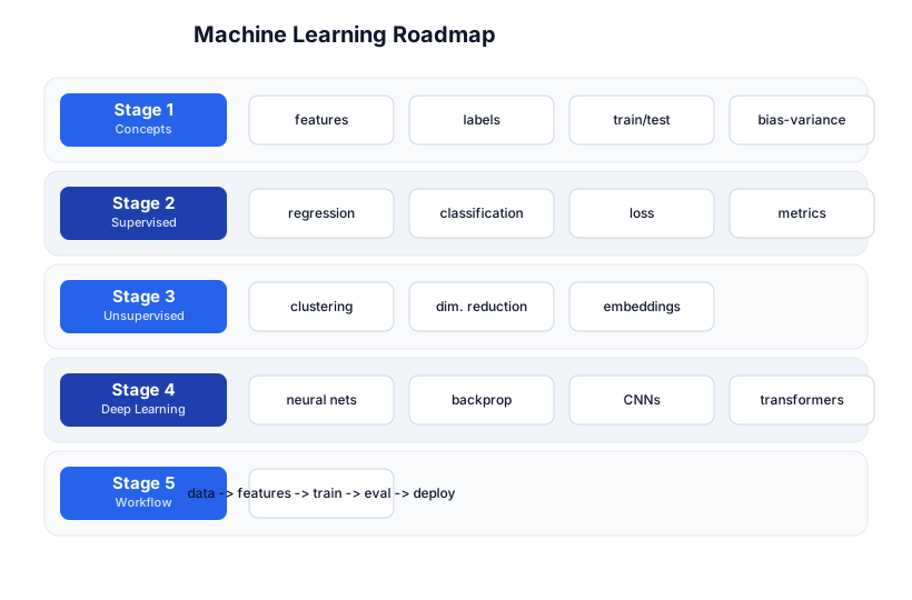
The roadmap moves from the core concepts (Stage 1), through the three paradigms (Stages 2-4), to the end-to-end workflow that ties them together (Stage 5). You’ll want Python and basic linear algebra as prerequisites.

---

Stage 1 — Core Concepts

What is machine learning?

A model is a function f(x) -> y that maps inputs (features) to outputs. Learning is the process of finding the f that best fits your data, by minimizing some measure of how wrong it is. You don’t write f by hand — you define a family of possible functions (linear, tree, neural net) and an optimization process searches for the best member of that family.

Features, labels, examples

• Example / sample — one data point (a row).
• Features (X) — the inputs: the things you measure. For a house: square footage, bedrooms, zip code.
• Label (y) — the output you’re predicting, if you have one: the house’s sale price.
• Dataset — a collection of (X, y) pairs (supervised) or just X (unsupervised).

Train / validation / test

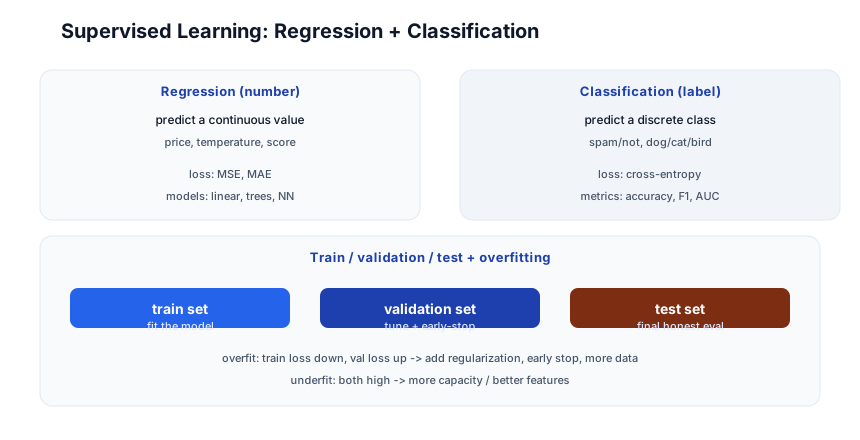
You train on one set of data, validate (tune) on another, and test (final honest evaluation) on a third you’ve never touched. The cardinal sin: evaluating on data you trained on — the model has memorized it, so the score is meaningless.

from sklearn.model_selection import train_test_split
X_train, X_test, y_train, y_test = train_test_split(X, y, test_size=0.2, random_state=42)

Bias-variance and overfitting

• Overfitting — the model fits the training data perfectly (memorizes noise) but fails on new data. Symptom: train loss goes down while validation loss goes up.
• Underfitting — the model is too simple; it can’t capture the pattern. Symptom: both losses are high.
• Bias-variance tradeoff — a model with high bias underfits (too rigid); high variance overfits (too flexible). The goal is the sweet spot: enough capacity to capture the pattern, not enough to memorize the noise.

Pitfall: Overfitting is the #1 beginner mistake. If your model gets 99% on training and 60% on validation, you overfit. Fixes: more data, simpler model, regularization (L1/L2), dropout (for NNs), early stopping.

---

Stage 2 — Supervised Learning

The paradigms

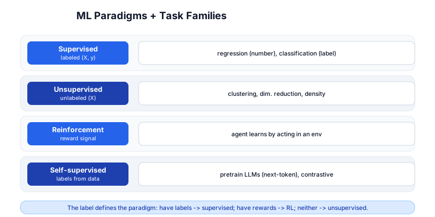
Supervised learning has labels. Two task types:

• Regression — predict a continuous number (house price, temperature). Loss: MSE (mean squared error), MAE.
• Classification — predict a discrete class (spam/not, dog/cat/bird). Loss: cross-entropy. Metrics: accuracy, precision/recall/F1, AUC.

A first model: linear regression

from sklearn.linear_model import LinearRegression
model = LinearRegression()
model.fit(X_train, y_train)         # "learn" the weights
predictions = model.predict(X_test)  # apply to new data

fit runs the optimization (ordinary least squares for linear regression) to find the weights that minimize MSE on the training set.

A first classifier: logistic regression

from sklearn.linear_model import LogisticRegression
model = LogisticRegression()
model.fit(X_train, y_train)
model.predict(X_test)           # predicted class
model.predict_proba(X_test)      # probability per class

Logistic regression is a classifier (despite the name): it outputs a probability via the sigmoid function, then thresholds.

The model zoo

Model	Good for	Notes
Linear / logistic regression	baselines, interpretable	the starting point; rarely the ending point
Decision trees	interpretable, non-linear	prone to overfit alone
Random forest / gradient boosting	tabular data, strong	the default for structured data; XGBoost/LightGBM win Kaggle
k-NN	small, simple	lazy; scales poorly
Naive Bayes	text, baselines	fast, independence assumption
Neural networks	images, text, audio	when data is unstructured and large

Pitfall: On tabular data (rows and columns), gradient-boosted trees (XGBoost, LightGBM) usually beat neural networks. Reach for deep learning when the data is unstructured (images, text, audio) or enormous. Don’t default to a neural net for a 50-column spreadsheet.

Metrics (classification)

from sklearn.metrics import accuracy_score, classification_report, confusion_matrix
accuracy_score(y_test, y_pred)               # fraction correct
print(classification_report(y_test, y_pred)) # precision, recall, F1 per class

• Accuracy — fraction correct. Misleading on imbalanced data (99% accuracy if 99% are one class).
• Precision — of predicted positives, how many are real? (avoid false alarms)
• Recall — of real positives, how many did we catch? (don’t miss cases)
• F1 — the harmonic mean of precision and recall (balance).
• AUC — area under the ROC curve; threshold-independent ranking quality.

Pitfall: Accuracy on an imbalanced dataset lies. If 1% of transactions are fraud, a model that always says “not fraud” is 99% accurate and useless. Use precision, recall, F1, or AUC.

---

Stage 3 — Unsupervised Learning

Unsupervised learning has no labels — you find structure in the data itself.

Clustering

k-means groups points into k clusters by minimizing within-cluster distance:

from sklearn.cluster import KMeans
kmeans = KMeans(n_clusters=5, random_state=42)
labels = kmeans.fit_predict(X)   # assign each point to a cluster

Other algorithms: DBSCAN (density-based, finds arbitrary shapes, no need to set k), hierarchical clustering (dendrogram).

Dimensionality reduction

PCA (principal component analysis) projects high-dimensional data onto fewer axes that capture the most variance — for visualization, compression, or as a preprocessing step:

from sklearn.decomposition import PCA
pca = PCA(n_components=2)
X_2d = pca.fit_transform(X)   # 100-dim -> 2-dim for plotting

Embeddings

An embedding is a learned dense vector representation of something (a word, a user, an image) where similar things are close in vector space. Word2vec, GloVe, and the embeddings inside transformers (Stage 4) turn discrete objects into continuous vectors so similarity (cosine distance) and analogies (“king - man + woman ≈ queen”) work. Embeddings are the foundation of modern search, recommendation, and LLMs — the pgvector extension in Postgres stores and searches them.

---

Stage 4 — Deep Learning

What a neural network is

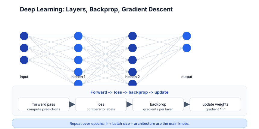
A neural network is a stack of layers; each layer is a linear transformation followed by a non-linear activation function. The “deep” in deep learning = many layers. Each layer learns progressively more abstract features: pixels → edges → shapes → parts → objects.

Forward pass, loss, backprop, update

Training is a loop:

1. Forward pass — push inputs through the layers, get predictions.
2. Loss — compare predictions to labels (MSE, cross-entropy).
3. Backpropagation — compute the gradient of the loss with respect to every weight, using the chain rule, layer by layer from output back to input.
4. Update — nudge each weight in the direction that reduces the loss: weight -= learning_rate * gradient (gradient descent).

Repeat over the whole dataset for many epochs. The main knobs: learning rate (step size — too big diverges, too small crawls), batch size (examples per update), and the architecture (how many layers, how wide).

A first neural net in PyTorch

import torch
import torch.nn as nn

model = nn.Sequential(
    nn.Linear(784, 128),   # input (28x28 pixels) -> 128
    nn.ReLU(),             # non-linear activation
    nn.Linear(128, 10),    # 128 -> 10 classes
)

loss_fn = nn.CrossEntropyLoss()
optimizer = torch.optim.Adam(model.parameters(), lr=1e-3)

for epoch in range(10):
    for X_batch, y_batch in dataloader:
        pred = model(X_batch)                    # forward
        loss = loss_fn(pred, y_batch)            # loss
        optimizer.zero_grad()
        loss.backward()                          # backprop (compute gradients)
        optimizer.step()                         # update weights

Architectures by data type

Data	Architecture	Why
Images	CNN (convolutional)	convolutions capture spatial patterns (edges, shapes) with few parameters
Sequences (text, time)	RNN/LSTM (legacy) → Transformer	transformers attend to all positions at once, parallelizable
Text (modern)	Transformer (GPT, BERT, Claude…)	self-attention; the architecture behind every LLM
Tabular	usually gradient boosting > NNs	trees handle structured data better

Pitfall: For most real problems, start simple (linear/logistic regression, then a tree model) and only reach for deep learning when you have unstructured data and enough of it. A neural net on a small tabular dataset usually loses to XGBoost and takes 10x longer to train.

---

Stage 5 — The ML Workflow

The end-to-end pipeline

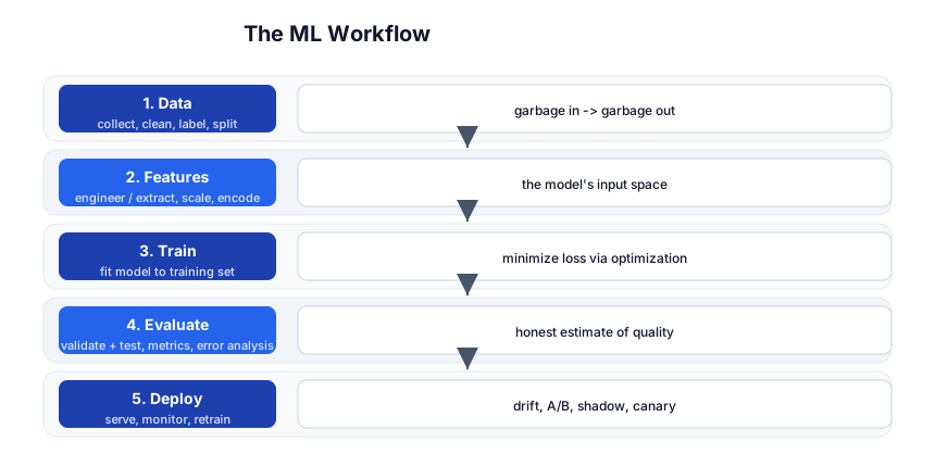
Building a model is ~20% of the work; the rest is the pipeline around it:

1. Data — collect, clean, label, split. “Garbage in, garbage out” is the #1 ML truth. Most ML time is spent here.
2. Features — transform raw data into what the model consumes: scale numerical features, encode categories (one-hot, embedding), handle missing values, create derived features.
3. Train — fit the model; tune hyperparameters (learning rate, tree depth) using the validation set.
4. Evaluate — report metrics on the test set (the one you never touched). Do error analysis: look at where it’s wrong, not just the aggregate score.
5. Deploy — serve the model (REST, batch, on-device). Monitor for drift — when the real-world data distribution shifts from training, accuracy silently degrades. Retrain on a schedule.

Pitfall: A model that scores great in a notebook but isn’t monitored in production will silently degrade as the world changes. Drift detection (track input distributions + prediction distributions over time) is how you catch it before users do.

Feature engineering and scaling

from sklearn.preprocessing import StandardScaler, OneHotEncoder
from sklearn.pipeline import Pipeline

pipeline = Pipeline([
    ('scaler', StandardScaler()),       # normalize numerical features to mean 0, std 1
    ('model', LogisticRegression()),
])
pipeline.fit(X_train, y_train)

Scale your features. Many models (linear, NNs, k-NN) behave badly when features are on different scales (a feature in millions dominates one in decimals). Tree models don’t care; everything else does.

Cross-validation

from sklearn.model_selection import cross_val_score
scores = cross_val_score(model, X, y, cv=5)   # 5-fold CV
print(scores.mean(), scores.std())

Cross-validation splits the data into k folds, trains on k-1 and validates on the held-out one, rotating — a more robust estimate of generalization than a single train/test split.

MLOps

The deployment + monitoring layer:

• Versioning — track which model version is serving (MLflow, Weights & Biases).
• Serving — REST endpoint (FastAPI + the model), batch scoring, or on-device.
• Monitoring — drift detection, prediction latency, input schema validation.
• Retraining — schedule retraining as data drifts; A/B test new models against the current one.

---

Quick-Start Checklist

1. Install scikit-learn + pandas — pip install scikit-learn pandas matplotlib.
2. Load a dataset — sklearn.datasets.load_iris() (classification) or load_diabetes() (regression).
3. Split train/test — always hold out a test set you never touch until the end.
4. Start with a baseline — logistic regression or a decision tree. Beat it before going complex.
5. Pick the metric for the problem — F1 for imbalanced classification, MSE for regression.
6. Cross-validate — don’t trust a single split.
7. Try gradient boosting (XGBoost/LightGBM) for tabular data — usually the winner.
8. Reach for PyTorch only when data is unstructured (images, text) or large.
9. Scale features for anything that isn’t a tree.
10. Set up drift monitoring before you ship — a model degrades silently.

Common Pitfalls

• Evaluating on training data — the model has seen it; the score is meaningless. Always hold out a test set.
• Overfitting — train loss down, val loss up. Regularize, get more data, or simplify.
• Accuracy on imbalanced data — misleading; use precision/recall/F1/AUC.
• Not scaling features — breaks linear models, NNs, k-NN; trees are immune.
• Data leakage — scaling/encoding on the whole dataset before splitting leaks test info into training. Fit preprocessors on train only; transform test with the fitted transformer (use a Pipeline).
• Defaulting to deep learning — for tabular data, trees usually win and train 10x faster.
• Ignoring drift — a great model in the notebook silently degrades in production as the world changes.
• No baseline — start with the simplest model; if a linear regression gets 90%, a neural net that gets 91% isn’t worth the complexity.

Further Reading

• Hands-On Machine Learning by Aurélien Géron — the standard practical book (scikit-learn + TensorFlow/Keras/PyTorch)
• scikit-learn User Guide — the docs are a tutorial
• PyTorch Tutorials — the deep-learning starting point
• Deep Learning Book by Goodfellow et al — the theory reference (free)
• Andrej Karpathy’s YouTube — “Let’s build GPT” etc., from first principles
• Papers With Code — state-of-the-art + implementations

Related guides

ML is the applied-math layer on top of programming fundamentals — these PyShine tutorials connect to it:

• Learn Python in One Post — the language every ML library uses; NumPy, pandas, scikit-learn, PyTorch are all Python.
• Learn Data Structures and Algorithms in One Post — Big-O and the fundamentals you need to reason about model complexity.
• Learn SQL in One Post — ML models train on data; most of it lives in a database.
• Learn PostgreSQL in One Post — the pgvector extension stores and searches ML embeddings.
• Learn Docker in One Post — containerize model training and serving.

---

Machine learning is less a single skill than a stack of decisions: what paradigm (supervised? unsupervised?), what model family (trees? neural nets?), what metric, what preprocessing, what monitoring. The five stages here — concepts, supervised, unsupervised, deep learning, the workflow — cover the whole map from “what is a feature” to “how do I detect drift in production.” The habit that separates a beginner from a practitioner is start with a baseline and beat it: a logistic regression or a tree, cross-validated, with the right metric, before you ever reach for a neural network. Load load_iris(), run the snippets above, and watch a model go from random to useful in ten lines — that’s the moment the field clicks.

Enjoyed this post? Never miss out on future posts by following us