Mixture of Experts: How LLMs Scale to Trillions Without Slowing Down

Every token you generate with GPT-4, DeepSeek-V3, or Mixtral activates only a fraction of the model’s parameters. A 671-billion-parameter model can run at the speed of a 37-billion-parameter model because not all parameters participate in every forward pass. This is not quantization, not distillation, not some clever kernel trick – it is Mixture of Experts (MoE), the sparse architecture that decouples model capacity (total parameters, i.e., knowledge) from inference cost (active parameters, i.e., compute per token).

In late 2023, Mistral AI released Mixtral 8x7B: 47 billion total parameters but only 13 billion active per token, matching or beating Llama 2 70B on benchmarks while running 4-6x faster. In December 2024, DeepSeek-V3 pushed the idea to 671 billion total parameters with just 37 billion active, achieving frontier-model quality at a fraction of the inference cost. Today, MoE is no longer a research curiosity – it is the default architecture for frontier-scale LLMs.

This post explains how MoE works, why it scales, what goes wrong during training (spoiler: routers love to play favorites), and how models like DeepSeek-V3 engineered around the problems. It follows our earlier posts on the attention mechanism, positional encoding, and building an LLM from scratch.

The Dense Scaling Wall

In a traditional “dense” transformer, every single parameter participates in every single forward pass for every single token. Each transformer block has two sublayers: a multi-head self-attention layer and a feed-forward network (FFN, also called MLP). The attention layer mixes information across tokens; the FFN processes each token independently through an up-projection, a non-linearity (typically SwiGLU in modern models), and a down-projection.

The FFN is where roughly two-thirds of the model’s parameters and compute live. For a hidden dimension D and FFN intermediate dimension F (typically F = 8D/3 in SwiGLU models), the FFN performs two matrix multiplications per token: D x F and F x D. That is 8D² multiply-adds per layer per token. To make the model smarter – to give it more knowledge, more linguistic patterns, more reasoning patterns – you widen D or add more layers, and the compute cost grows proportionally.

This creates a brutal trade-off:

Model	Total params	Active params/token	Relative FLOPs
Llama 2 7B	7B	7B	1x
Llama 2 70B	70B	70B	10x
Mixtral 8x7B	47B	13B	~1.8x
DeepSeek-V3	671B	37B	~5x

A dense 70B model needs 10x more compute per token than a 7B model. Mixtral 8x7B has more parameters than a 70B model but needs less compute per token than a 13B model. That is the promise of sparsity: you can have a library of a million books without reading every book to answer every question.

The Core Idea: Sparse Activation

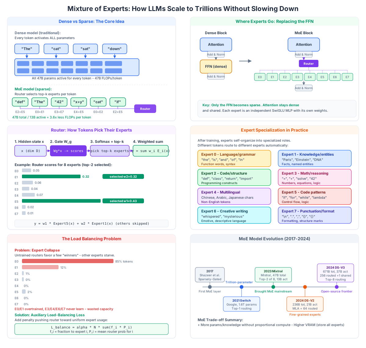
The mental model is a library. A dense model reads every book in the library to answer every question. A MoE model has a librarian (the router) who quickly selects a small number of relevant books (experts), reads only those, and combines what they say. The library (total parameters) can be enormous, but the reading time (compute per token) stays small.

Instead of one large FFN in each transformer block, an MoE block places N smaller FFNs – called experts – in parallel, plus a lightweight router (or gate) network that decides which experts should process each token. The router picks the top k experts for each token, sends the token through only those experts, and combines their outputs with a weighted sum.

For Mixtral 8x7B, N = 8 experts and k = 2 – each token activates 2 out of 8 experts. For DeepSeek-V3, N = 256 routed experts plus 1 shared expert, and k = 8.

Crucially, only the FFN becomes sparse. The self-attention layers remain dense and shared across all tokens. The attention mechanism needs to see the entire sequence to compute attention weights; making it sparse would break the core computation. But the FFN is embarrassingly per-token, making it the natural place to introduce expert routing.

Anatomy of an MoE Layer

Let us trace what happens to a single token as it passes through an MoE layer.

Step 1: The Router Computes Scores

The router is a single linear layer: scores = W_g · x, where x is the token’s hidden state (dimension D) and W_g is a learned weight matrix of shape (D, N) that projects to one score per expert. This is followed by a softmax to convert scores to probabilities across experts:

p = softmax(scores)    # shape (N,)

Step 2: Top-k Selection

The router selects the k experts with the highest probabilities. For Mixtral, k = 2; for Switch Transformer, k = 1; for DeepSeek-V3, k = 8. The probabilities for the selected experts are re-normalized so they sum to 1, giving weights w_1, w_2, ..., w_k.

All unselected experts are completely skipped. Their weights are not loaded, not computed, not touched. This is where the compute savings come from.

Step 3: Expert Computation

The token’s hidden state is dispatched to each of the k selected experts. Each expert is an independent SwiGLU FFN with its own set of weights. The expert computes an output: y_i = Expert_i(x) for each selected expert i.

Step 4: Weighted Combination

The outputs are combined using the router weights:

y = w_1 * Expert_1(x) + w_2 * Expert_2(x) + ... + w_k * Expert_k(x)

This weighted sum becomes the output of the MoE layer, which is then passed through the residual connection and layer norm just like a regular FFN output.

Minimal PyTorch Implementation

Here is a simplified MoE FFN that illustrates the core logic. This is for clarity – real implementations use grouped GEMMs, expert parallelism, and capacity-based batching for efficiency:

import torch
import torch.nn as nn
import torch.nn.functional as F

class Expert(nn.Module):
    """A single SwiGLU FFN expert."""
    def __init__(self, dim: int, hidden_dim: int):
        super().__init__()
        self.w1 = nn.Linear(dim, hidden_dim, bias=False)
        self.w2 = nn.Linear(hidden_dim, dim, bias=False)
        self.w3 = nn.Linear(dim, hidden_dim, bias=False)  # SwiGLU gate

    def forward(self, x: torch.Tensor) -> torch.Tensor:
        return self.w2(F.silu(self.w1(x)) * self.w3(x))


class MoELayer(nn.Module):
    """Simplified Mixture of Experts FFN layer."""
    def __init__(self, dim: int, hidden_dim: int, num_experts: int = 8, top_k: int = 2):
        super().__init__()
        self.num_experts = num_experts
        self.top_k = top_k
        self.gate = nn.Linear(dim, num_experts, bias=False)
        self.experts = nn.ModuleList([
            Expert(dim, hidden_dim) for _ in range(num_experts)
        ])

    def forward(self, x: torch.Tensor) -> torch.Tensor:
        # x shape: (batch, seq_len, dim)
        B, T, D = x.shape
        x_flat = x.view(-1, D)  # (B*T, D)

        # Step 1: Router scores
        router_logits = self.gate(x_flat)  # (B*T, num_experts)
        router_probs = F.softmax(router_logits, dim=-1)

        # Step 2: Select top-k experts
        top_weights, top_indices = torch.topk(router_probs, self.top_k, dim=-1)
        top_weights = top_weights / top_weights.sum(dim=-1, keepdim=True)  # renormalize

        # Step 3+4: Dispatch to experts and combine
        out = torch.zeros_like(x_flat)
        for expert_idx in range(self.num_experts):
            # Find tokens routed to this expert
            mask = (top_indices == expert_idx).any(dim=-1)  # (B*T,)
            if not mask.any():
                continue
            expert_input = x_flat[mask]
            expert_output = self.experts[expert_idx](expert_input)
            # Weight by routing probability for each k slot
            for k_slot in range(self.top_k):
                slot_mask = mask & (top_indices[:, k_slot] == expert_idx)
                if slot_mask.any():
                    out[slot_mask] += top_weights[slot_mask, k_slot:k_slot+1] * self.experts[expert_idx](x_flat[slot_mask])

        return out.view(B, T, D)

Real implementations (like Megablocks, DeepSeek’s custom kernels, or vLLM’s MoE backend) avoid the Python loop over experts. They use a “permute → batch GEMM → unpermute” pattern: tokens are gathered by expert ID into contiguous batches, each expert processes its batch in one large matrix multiplication, and the outputs are scattered back to their original positions. This yields dramatically better GPU utilization.

Expert Specialization

After training, experts automatically self-organize into specialized roles. The router learns to send different types of tokens to different experts, and each expert becomes better at processing the tokens it consistently receives.

Studies of trained MoE models (most notably the Mixtral paper [2]) have found that experts specialize in predictable patterns:

• Syntax experts specialize in function words: “the”, “is”, “and”, “of”, “in”
• Knowledge experts specialize in named entities and factual content: “Paris”, “Einstein”, “DNA”
• Code experts specialize in programming constructs: “def”, “class”, “return”, “import”, “if”, “for”
• Math experts specialize in numbers and reasoning: “=”, “+”, “solve”, numeric tokens
• Multilingual experts specialize in non-English scripts: Chinese characters, Arabic, Japanese
• Punctuation experts specialize in formatting tokens: newlines, brackets, commas

This specialization is entirely emergent – nothing in the architecture explicitly assigns roles to experts. It is a natural consequence of the load-balancing pressure plus the router learning to minimize loss. Code tokens consistently sent to expert 2 will cause expert 2’s gradients to specialize toward code representations, which in turn makes the router even more likely to send code tokens to expert 2, creating a reinforcing feedback loop.

This specialization is why MoE models can learn more effectively than dense models of the same active parameter count: each expert can afford to be a narrow specialist rather than a generalist forced to compress all knowledge into one FFN.

The Load Balancing Problem

If you train the naive MoE described above, it will fail. The router will quickly converge to sending almost all tokens to a small handful of experts. The favored experts get well-trained, which makes them even more favored (since they produce lower loss), while the ignored experts receive no gradient signal and remain essentially random. This is called expert collapse, and it is the fundamental training challenge for MoE.

Why Collapse Happens

The router’s objective is to minimize the language modeling loss. If expert 3 happens to produce slightly better outputs early in training, the router increases the probability of routing to expert 3, which gives expert 3 more training signal, making it even better, and so on. This is a positive feedback loop that leads to a few “winner” experts processing 80-90% of all tokens while the rest starve. The model effectively wastes the capacity of the unused experts.

Auxiliary Load-Balancing Loss

The fix, introduced by Shazeer et al. [1] and refined in Switch Transformer [3], is to add an auxiliary loss term that penalizes uneven expert assignment:

L_balance = alpha * N * sum_i(f_i * P_i)

where:

• N is the number of experts
• f_i is the fraction of tokens dispatched to expert i in the current batch
• P_i is the mean router probability assigned to expert i across all tokens
• alpha is a small coefficient (typically 0.01 to 0.001)

This loss is minimized when both f_i and P_i are uniform (1/N for all experts). It jointly penalizes dispatching too many tokens to one expert (high f_i) and assigning high router probabilities to one expert (high P_i). The total training loss becomes L_total = L_LM + L_balance.

Capacity Factor

In addition to the auxiliary loss, implementations use a capacity factor to enforce a hard limit on how many tokens each expert can process in a batch:

capacity_per_expert = (B * T / N) * capacity_factor

where capacity_factor is typically around 1.25 (meaning each expert can handle up to 25% more than its “fair share”). Tokens that would overflow an expert’s capacity are either dropped (sent via the residual connection without expert processing) or routed to a backup expert. This prevents GPU memory overflow and ensures balanced computation across distributed devices.

Shared Experts

DeepSeek-V3 [5] introduced a key refinement: shared experts. In addition to the 256 routed experts, each MoE layer includes 1 shared expert that processes every token unconditionally. The shared expert captures common, universal patterns (like basic syntax and frequent token combinations) that should not be routed, while the routed experts handle specialized knowledge. The output becomes:

y = SharedExpert(x) + sum_i(w_i * RoutedExpert_i(x))

This design choice reduces the routing burden on the most common tokens and improves stability, while still providing the benefits of fine-grained specialization for the routed experts.

MoE Through Time

Let us trace how MoE evolved from a research idea to the dominant architecture for frontier models.

2017: Sparsely-Gated MoE (Shazeer et al.)

The original MoE layer was introduced by Shazeer et al. at Google in “Outrageously Large Neural Networks” [1]. They demonstrated that a language model with 137 billion parameters using 10K experts (with top-2 routing) could achieve better perplexity than a dense baseline with a fraction of the compute. However, the approach was limited to a per-token routing mechanism that was difficult to scale in distributed training, and it took several years for the systems infrastructure to catch up.

2021: Switch Transformer (Fedus et al., Google)

Google’s Switch Transformer [3] simplified routing to top-1 (each token goes to exactly one expert) and scaled to 1.6 trillion parameters – the first trillion-parameter language model. They introduced the auxiliary load-balancing loss and selective precision training to stabilize large-scale MoE. Despite the impressive scale, Switch models were not released openly, and the architecture remained largely confined to Google’s infrastructure.

2023: Mixtral 8x7B (Mistral AI)

Mixtral 8x7B [2], released in December 2023, brought MoE to the open-source community. With 47 billion total parameters (8 experts of ~7B each, though actual parameter count is ~47B not 56B due to shared attention layers), top-2 routing, and 13 billion active parameters per token, Mixtral matched or outperformed Llama 2 70B and GPT-3.5 on most benchmarks while running at the speed of a 13B model. Crucially, it was released as open weights and worked with standard inference frameworks, making MoE accessible to everyone.

2024: DeepSeek-V2 and V3

DeepSeek-V2 (May 2024) [4] introduced Multi-head Latent Attention (MLA) to reduce KV-cache memory and scaled MoE to 236 billion total parameters with 21 billion active per layer, using 64 routed experts. DeepSeek-V3 (December 2024) [5] pushed further to 671 billion total parameters with 37 billion active, using:

• 256 fine-grained routed experts (smaller, more numerous experts than Mixtral’s 8)
• 1 shared expert always active (absorbing common patterns)
• Top-8 routing (more experts per token, enabling finer composition)
• Auxiliary-loss-free load balancing using a complementary sequence-wise bias

DeepSeek-V3 demonstrated that a 671B MoE could be trained on just 2.788 million H800 GPU hours (a fraction of what dense frontier models cost) while matching closed models like GPT-4o and Claude 3.5 Sonnet on many benchmarks. It was a watershed moment showing that MoE + careful systems engineering could deliver frontier quality at radically lower cost.

2025 and Beyond

Qwen3-MoE, Llama 4 Scout/Maverick, Grok, and the open GPT-OSS-120B all use MoE architectures. The trend is clear: more experts, finer granularity, auxiliary innovations like shared experts, and better systems for expert parallelism. The dense scaling era for frontier models is effectively over.

Inference Challenges

MoE introduces systems challenges that dense models do not face:

Expert Parallelism

Since each expert processes a different subset of tokens, experts can be distributed across multiple GPUs. This is called expert parallelism (EP). For DeepSeek-V3, the 256 experts per layer can be sharded across many GPUs – a typical deployment uses EP=320 (experts spread across 320 GPU ranks) for the MoE layers, while attention layers use tensor parallelism (TP=4).

All-to-All Communication

When experts are distributed across GPUs, tokens must be sent to the GPU holding their selected experts, and the outputs must be sent back. This is an all-to-all communication pattern that is expensive on standard networking. DeepSeek and other MoE deployments rely on high-bandwidth interconnects (InfiniBand, NVLink) and custom communication kernels to hide this latency.

Memory Trade-off

MoE models require more VRAM than a dense model of the same active parameter count. You must store all expert weights in memory even though only a fraction are active per token. Mixtral 8x7B needs ~90GB in FP16 (similar to a dense 70B), despite running at 13B speed. MoE trades memory for speed: you spend more memory to get faster inference with more total knowledge.

Batch Effects

In dense models, larger batches improve GPU throughput monotonically. In MoE models, the routing pattern varies per token, which can lead to load imbalance across GPUs in a batch. Advanced batching strategies (like continuous batching used in vLLM and SGLang) and expert-aware scheduling are required to achieve good throughput.

When to Use MoE (and When Not To)

MoE is not a free lunch. It makes sense when:

• You need frontier-level capability and can afford the multi-GPU deployment
• You want to scale knowledge capacity without proportional inference cost
• You have the systems infrastructure for expert parallelism and high-bandwidth communication

Dense models remain preferable when:

• You are deploying on a single GPU or consumer hardware (the memory overhead is prohibitive)
• You need simple, predictable latency (MoE has variable latency due to routing and communication)
• You are fine-tuning a small specialist model (7B-14B dense is usually better than 47B MoE for narrow tasks)

For many practical use cases – especially local inference on a single GPU – well-quantized dense models (as discussed in our quantization post) remain the best choice. But at the frontier, MoE is now the default.

Practical Takeaways

1. MoE replaces the FFN, not attention. Self-attention stays dense; only the feed-forward network is split into experts. If someone says “MoE attention,” they are almost always talking about something experimental.

2. Top-k selection with k=2 is the sweet spot for quality vs cost. Switch Transformer used k=1 for simplicity; Mixtral used k=2; DeepSeek-V3 uses k=8 with fine-grained experts. Higher k gives better quality but costs more compute.

3. Load balancing is not optional. Without auxiliary loss (or DeepSeek-V3’s bias-based alternative), routers collapse. Expect to see 1-2 experts taking 50%+ of tokens if you skip it.

4. More experts + smaller experts (fine-grained MoE) is the modern trend. DeepSeek-V3’s 256 small experts outperform Mixtral’s 8 large experts per active parameter. The routing overhead is amortized, and specialization is sharper.

5. MoE inference is memory-bound, not compute-bound. You need more VRAM than a dense model of equivalent speed. The main cost is holding all expert weights.

6. Shared experts improve stability. Adding one always-active shared expert captures universal patterns and reduces the routing load on common tokens. This is a simple, effective technique that will likely become standard.

Summary

Mixture of Experts breaks the fundamental assumption that model capacity must cost proportional compute. By replacing the FFN with a pool of parallel experts and a learned router, MoE models can store vastly more knowledge while keeping inference costs manageable. The architecture has evolved rapidly from Shazeer’s 2017 proposal to Switch Transformer’s trillion-parameter proof of concept, to Mixtral’s open-source breakthrough, to DeepSeek-V3’s production-grade 671B model with 256 fine-grained experts.

The challenges – expert collapse, all-to-all communication, memory overhead – are real but increasingly well-understood. As of 2026, every major frontier model uses MoE or a similar sparse mechanism. Understanding how it works is no longer optional for anyone working with LLMs at scale.

References

[1] Shazeer, N. et al. “Outrageously Large Neural Networks: The Sparsely-Gated Mixture-of-Experts Layer.” ICLR 2017. arXiv:1701.06538

[2] Jiang, A.Q. et al. “Mixtral of Experts.” 2024. arXiv:2401.04088

[3] Fedus, W., Zoph, B., Shazeer, N. “Switch Transformers: Scaling to Trillion Parameter Models with Simple and Efficient Sparsity.” JMLR 2022. arXiv:2101.03961

[4] DeepSeek-AI. “DeepSeek-V2: A Strong, Economical, and Efficient Mixture-of-Experts Language Model.” 2024. arXiv:2405.04434

[5] DeepSeek-AI. “DeepSeek-V3 Technical Report.” 2024. arXiv:2412.19437

Enjoyed this post? Never miss out on future posts by following us