LLM Attention Mechanism: The Heart of the Transformer

If the transformer is the engine of modern AI, attention is its combustion chamber. Every breakthrough in large language models – from GPT to Llama to Gemini – is built on the same fundamental operation: self-attention. Despite its centrality, attention is often explained either too abstractly (with analogies that obscure the mechanics) or too mathematically (with equations that hide the intuition).

This post traces attention from first principles. We will cover what Q, K, and V actually represent, why multi-head attention exists, how grouped-query attention (GQA) reduces the KV-cache bottleneck we discussed in our previous post, and why causal masking is essential for autoregressive generation. This is the fourth post in our LLM internals series, following tokenization (which produces the embeddings that attention consumes).

Self-Attention: The Core Operation

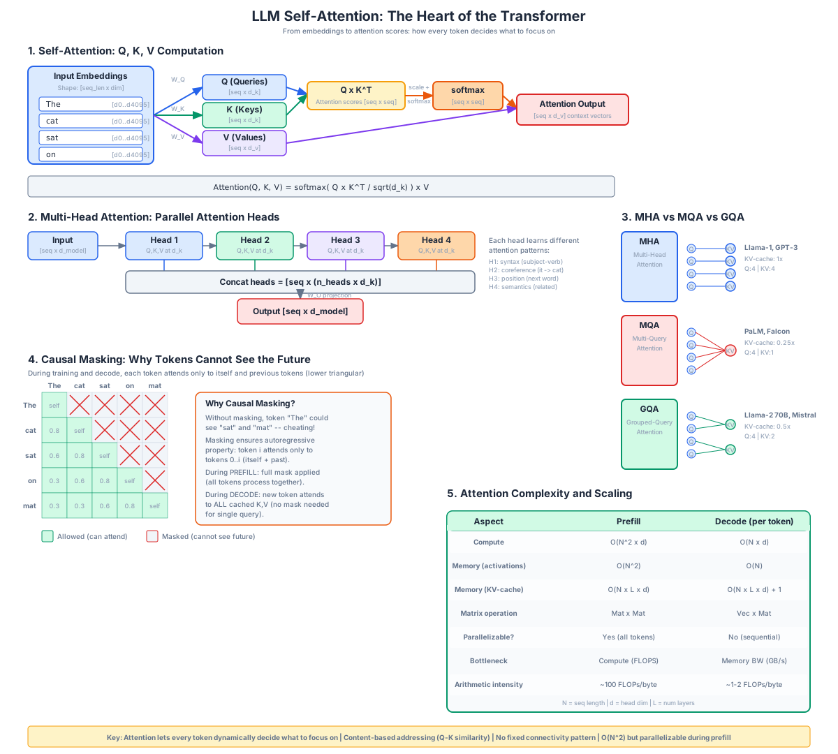
Understanding the Diagram

The diagram above breaks down the attention mechanism into six interconnected sections. Let us examine each in detail.

Section 1: Self-Attention – Q, K, V Computation

The left section shows the complete self-attention pipeline for a single attention head. The process begins with input embeddings – the output of the tokenization pipeline we covered in the previous post. Each token has been converted to a dense vector of dimension d_model (typically 4096 for a 7B model).

Query, Key, Value Projections Each input embedding is multiplied by three learned weight matrices – W_Q, W_K, and W_V – to produce three new vectors for each token: the Query (Q), Key (K), and Value (V). These projections are the model’s way of extracting three different “views” of each token:

• Query (Q): “What am I looking for?” – This vector encodes what information the current token needs from other tokens.
• Key (K): “What do I contain?” – This vector encodes what information this token offers to others.
• Value (V): “If you select me, here is my contribution” – This vector is the actual content that gets passed along if the attention weight is high.

The projection matrices W_Q, W_K, and W_V are learned during training. They transform the generic embedding into specialized roles. The dimensionality is reduced from d_model to d_k (typically d_model / num_heads = 4096/32 = 128) to keep the computation manageable.

Attention Score Computation (Q x K^T) The attention scores are computed by taking the dot product of each token’s Query with every token’s Key. This produces an N x N matrix (where N is the sequence length) where entry (i, j) represents how strongly token i should attend to token j. A high score means “token i finds token j relevant.”

The dot product is a natural similarity measure: vectors pointing in similar directions produce high scores. This is why attention is sometimes called “content-based addressing” – the Query “queries” the Keys, and the most similar Keys get the highest attention weights.

Scaling and Softmax The raw scores are divided by sqrt(d_k) to prevent the values from growing too large (which would push softmax into regions with vanishing gradients). Then softmax is applied across each row, converting scores into probabilities that sum to 1. This ensures the attention weights form a valid probability distribution.

Weighted Sum (softmax x V) The attention probabilities are multiplied by the Value matrix, producing a weighted average of all tokens’ Values. Tokens with high attention weights contribute more to the output; tokens with low weights contribute less. The result is a context-aware representation of each token – one that has incorporated information from all relevant tokens in the sequence.

The Attention Formula The entire operation is captured in one elegant equation:

Attention(Q, K, V) = softmax(Q x K^T / sqrt(d_k)) x V

This single formula, introduced in the “Attention Is All You Need” paper, is the mathematical heart of every modern LLM.

Section 2: Multi-Head Attention

A single attention head can only learn one type of relationship. But language has many different types of relationships – syntactic (subject-verb agreement), semantic (coreference: “it” refers to “cat”), positional (next word prediction), and structural (paragraph-level coherence).

Multi-head attention solves this by running multiple attention heads in parallel, each with its own Q, K, V projections. The diagram shows four heads, each learning a different attention pattern:

• Head 1: Syntax – attending to grammatically related tokens (subject attends to verb)
• Head 2: Coreference – attending to referent tokens (“it” attends to “cat”)
• Head 3: Position – attending to nearby tokens (sequential context)
• Head 4: Semantics – attending to conceptually related tokens

Each head operates on a reduced dimension d_k = d_model / num_heads. The outputs of all heads are concatenated and multiplied by an output projection matrix W_O, producing the final output with the same dimension as the input.

For Llama-2 7B: d_model = 4096, num_heads = 32, d_k = 128. Each head processes 128-dimensional Q, K, V vectors, and the 32 heads’ outputs are concatenated back to 4096 dimensions.

Section 3: MHA vs MQA vs GQA

The right section compares three attention variants that differ in how many Key and Value heads they use:

Multi-Head Attention (MHA) The original design: every query head has its own K and V head. If there are H query heads, there are also H KV heads. This provides maximum expressiveness but means the KV-cache (which stores K and V for all heads) is at its largest. For Llama-2 7B with 32 heads, each token’s KV-cache occupies 0.5 MB. GPT-3 and the original Transformer use MHA.

Multi-Query Attention (MQA) Introduced by Shazeer in 2019, MQA uses multiple query heads but only a SINGLE shared K and V head. All query heads attend to the same keys and values. This reduces the KV-cache by a factor of H (e.g., 32x for Llama-2 7B), dramatically improving decode speed. However, quality degrades because the model loses the ability to compute different K, V representations for different heads. PaLM and Falcon use MQA.

Grouped-Query Attention (GQA) Introduced by Ainslie et al. in 2023, GQA is the sweet spot between MHA and MQA. Query heads are divided into G groups, and each group shares a single K and V head. When G = H, it is MHA; when G = 1, it is MQA. The typical choice is G = 8, which reduces the KV-cache by 8x while maintaining quality close to MHA.

GQA is the industry standard as of 2026: Llama-2 70B, Llama-3 (all sizes), Mistral, Mixtral, and Gemma all use GQA with 8 KV groups. The quality-speed tradeoff is favorable because the KV-cache reduction directly addresses the memory-bandwidth bottleneck of decode (as explained in our KV-cache deep dive).

For Llama-2 70B (80 layers, 64 query heads, 8 KV heads, 128 dim): each token’s KV-cache is 2 x 2 x 80 x 8 x 128 = 327,680 bytes = 0.33 MB, compared to 2.62 MB with MHA. At 32K context, this saves 73 GB of VRAM per request.

Section 4: Causal Masking

The bottom-left section shows the causal masking matrix – a critical component that prevents tokens from “seeing the future.” The 5x5 grid shows which token pairs are allowed to attend to each other:

• Green cells (lower triangle): Token i CAN attend to token j (where j <= i). “sat” can attend to “The”, “cat”, and itself.
• Red X (upper triangle): Token i CANNOT attend to token j (where j > i). “cat” cannot attend to “sat” or “on”.

Without causal masking, the model could cheat during training by looking ahead at future tokens. This would make training trivially easy but would break autoregressive generation – at inference time, future tokens do not exist yet.

During prefill (prompt processing), causal masking is applied to the full N x N attention matrix. During decode, the single new token’s query attends to ALL cached K, V values – no masking is needed because all cached tokens are in the past.

Section 5: Attention Complexity

The bottom-right table compares the computational complexity of attention during prefill vs decode:

• Prefill: O(N^2 x d) compute and O(N^2) memory for the attention matrix. All N tokens are processed in parallel, making this compute-bound.
• Decode: O(N x d) compute per token. The single query vector attends to N cached K, V values. This is memory-bandwidth-bound because the entire KV-cache must be loaded for each token.

The O(N^2) complexity of prefill is why processing a 100K-token prompt takes significantly longer than a 1K-token prompt. The linear O(N) complexity of decode (per token) is why each output token is fast individually but the total decode time scales linearly with output length.

How Attention Heads Learn Different Patterns

Research into attention head interpretability has revealed that different heads naturally specialize for different linguistic tasks:

Syntactic Heads: Some heads consistently attend from verbs to their subjects and objects. For example, in “The cat that the dog chased ran away”, a syntactic head will have “ran” attend directly to “cat” (skipping the relative clause).

Coreference Heads: Certain heads track pronoun references. In “The cat sat on the mat because it was tired”, a coreference head will have “it” attend to “cat” with high weight.

Positional Heads: Some heads are primarily driven by position rather than content. They attend to the immediately preceding token, the token two positions back, or other fixed offsets. These heads help the model track word order.

Rare Word Heads: Some heads specialize in attending to rare or unusual tokens, helping the model incorporate information from unusual vocabulary.

This specialization emerges naturally from training – no explicit instruction tells heads what to specialize in. The multi-head architecture provides the capacity for diverse attention patterns, and gradient descent discovers which specializations are useful for language modeling.

The O(N^2) Problem and Why It Matters

The attention computation requires an N x N matrix (where N is the sequence length) because every token must compute its similarity with every other token. This quadratic scaling is the fundamental limitation of the Transformer architecture:

• N = 1,000: 1 million attention scores (manageable)
• N = 10,000: 100 million scores (significant memory)
• N = 100,000: 10 billion scores (requires special techniques)
• N = 1,000,000: 1 trillion scores (requires architectural changes)

This is why extending context windows beyond 128K tokens is difficult. The attention matrix alone for 1M tokens in FP16 would consume 2 TB of memory – far exceeding any GPU’s VRAM.

Several approaches address this:

• FlashAttention: Does not reduce the O(N^2) complexity but avoids materializing the full matrix in HBM, reducing memory from O(N^2) to O(N)
• Sliding Window Attention: Each token only attends to a local window of W tokens, reducing to O(N x W)
• Sparse Attention: Only attend to selected token pairs based on patterns, reducing to O(N x k)
• Linear Attention: Approximate attention with kernel functions, achieving O(N) complexity
• State Space Models (Mamba, RWKV): Replace attention entirely with recurrent structures that have O(1) memory per step

GQA: Why It Became the Industry Standard

The transition from MHA to GQA is one of the most impactful architectural changes in recent LLM history. Here is why:

The Problem with MHA: The KV-cache grows with both sequence length and the number of attention heads. For a 70B model with 64 heads, each token requires 2.6 MB of KV-cache. At 32K context, that is 85 GB – more than two A100 40GB GPUs can hold.

The Problem with MQA: While MQA reduces the KV-cache by 64x, it degrades quality because all 64 query heads must share the same K and V representations. Different heads cannot learn different key-value patterns, limiting the model’s expressiveness.

The GQA Solution: By using 8 KV groups (instead of 64 or 1), GQA achieves an 8x KV-cache reduction while maintaining quality within 1% of MHA. The key insight is that most attention heads within a group learn similar patterns, so sharing K, V projections within a group loses little information.

Uptraining: Ainslie et al. showed that existing MHA checkpoints can be converted to GQA with only 5% of the original pretraining compute. This means models do not need to be trained from scratch – they can be “uptrained” to GQA cheaply.

Industry Adoption: As of 2026, virtually all open-weight LLMs use GQA with 8 groups: Llama-2 70B, Llama-3 (8B, 70B, 405B), Mistral 7B, Mixtral 8x7B, and Gemma 2. This convergence on GQA-8 represents the empirical consensus that 8 KV groups is the optimal quality-speed tradeoff.

Practical Implications

For model selection: If you are choosing between models for a memory-constrained deployment, GQA models can serve more concurrent requests. A Llama-2 70B (GQA-8) can serve roughly 8x more concurrent requests than a hypothetical MHA version at the same context length.

For inference optimization: GQA is complementary to other optimizations. You can combine GQA (reduces KV-cache size) with FlashAttention (reduces HBM accesses) and KV-cache quantization (reduces precision) for multiplicative improvements. Modern inference servers like vLLM and TensorRT-LLM support all three simultaneously.

For training cost: The GQA uptraining recipe means you can train with MHA (slightly higher quality during training) and convert to GQA for deployment, getting the best of both worlds for only 5% additional compute.

For context window extension: GQA’s KV-cache reduction is a necessary (but not sufficient) condition for long context windows. Without GQA, a 128K context on a 70B model would require 340 GB of KV-cache – impossible on any single GPU. With GQA-8, it requires 42 GB, which fits on an A100 80GB.

Further Reading

• Attention Is All You Need (Vaswani et al., 2017) – The paper that introduced self-attention and the Transformer architecture
• Fast Transformer Decoding: One Write-Head is All You Need (Shazeer, 2019) – The Multi-Query Attention (MQA) paper
• GQA: Training Generalized Multi-Query Transformer Models (Ainslie et al., 2023) – The Grouped-Query Attention paper
• FlashAttention: Fast and Memory-Efficient Exact Attention (Dao et al., 2022) – IO-aware attention that reduces HBM accesses

Related Posts

• LLM Tokenization: How Text Becomes Numbers
• LLM Decode Deep Dive: KV-Cache, GPU VRAM, and the Memory Bottleneck
• LLM Prompt vs Decode: Understanding the Two Phases of LLM Inference

Conclusion

Self-attention is the operation that makes the Transformer powerful. By computing Query-Key similarity, the model dynamically decides which tokens to focus on for each position. Multi-head attention extends this by running parallel heads that specialize in different linguistic phenomena – syntax, coreference, position, semantics.

The evolution from MHA to MQA to GQA reflects the practical reality of LLM deployment: the KV-cache bottleneck (covered in our previous post) is so severe that reducing the number of K, V heads became the single most impactful architectural change. GQA-8 is now the industry standard because it achieves 8x KV-cache reduction with negligible quality loss, and the uptraining recipe makes it accessible to existing MHA checkpoints.

Causal masking completes the picture by ensuring the model cannot peek at future tokens during training – a seemingly simple constraint that is essential for autoregressive generation. Without it, the model would learn to depend on future information that does not exist at inference time.

Together, these components – self-attention, multi-head parallelism, GQA efficiency, and causal masking – form the attention mechanism that powers every modern LLM. Understanding them is essential for anyone who wants to go beyond using LLMs as black boxes and start optimizing, customizing, or building with them.

Enjoyed this post? Never miss out on future posts by following us