Positional Encoding: How LLMs Know Word Order Without Recurrence

Recurrent neural networks processed tokens one at a time, left to right. The order of words was baked into the computation graph. When the Transformer [1] replaced recurrence with self-attention in 2017, it gained parallelism and long-range gradient flow – but it lost something fundamental: self-attention is permutation-equivariant. Shuffle the input tokens, and the attention scores stay the same. “Dog bites man” produces the same activations as “Man bites dog” unless you explicitly tell the model which position each token occupies.

Positional encoding is how we inject that information. It is the mechanism by which every modern LLM – GPT, Llama, Mistral, Gemini, Qwen – knows word order. The approach has evolved dramatically since 2017, and the differences between the four major schemes (sinusoidal, learnable, RoPE, ALiBi) directly determine how long your context window can be, whether you can extrapolate to unseen sequence lengths at inference time, and how much fine-tuning you need to scale from 4K to 128K tokens.

This post walks through all four methods, explains why RoPE won, and then dives into the scaling tricks (Position Interpolation, NTK-aware scaling, YaRN) that gave us million-token context windows in 2024. It follows naturally from our earlier pieces on the attention mechanism and building an LLM from scratch.

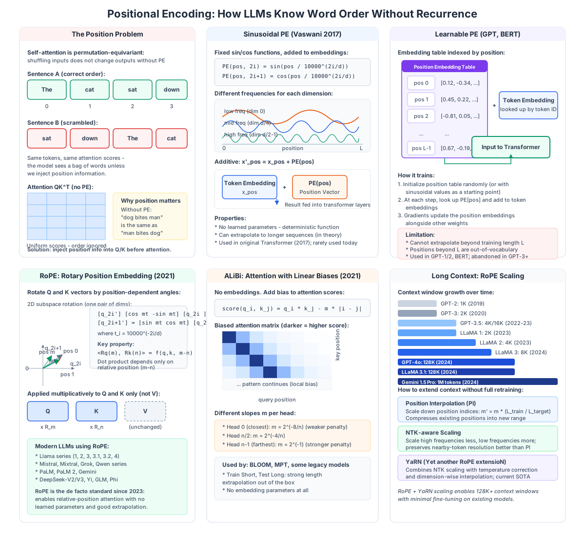
The Position Problem

Self-attention computes, for every pair of tokens (i, j), an attention weight from their dot product: \[\text{Attention}(Q, K, V) = \text{softmax}\left(\frac{QK^T}{\sqrt{d_k}}\right)V\]

The weight between token i and token j depends only on the content vectors $q_i$ and $k_j$, not on where either token sits in the sequence. Without modification, the attention pattern for “The cat sat” is identical to “sat cat The” – the model sees a bag of words.

You can see this in the uniform attention scores in panel 1 of the diagram above: every cell in the QK^T matrix has the same value, because the keys and queries contain no positional signal. This is not a bug in the math; it is by design. Permutation equivariance is what makes self-attention so expressive and so easy to parallelize. It just means that position has to be injected separately, before attention is computed.

The question is how. The answer has gone through three generations.

First Generation: Fixed and Learnable Embeddings (2017-2019)

Sinusoidal Positional Encoding (Vaswani et al., 2017)

The original Transformer paper proposed a deterministic, non-learned function. For each position pos and each dimension pair (2i, 2i+1): \[\begin{align*} PE(pos, 2i) &= \sin\left(pos / 10000^{2i/d}\right) \\ PE(pos, 2i+1) &= \cos\left(pos / 10000^{2i/d}\right) \end{align*}\]

Each dimension gets a sinusoid of a different frequency, as shown in panel 2. Dimension 0 has a wavelength of $2\pi \cdot 10000^0 \approx 6.3$ – it oscillates wildly from one token to the next. Dimension d/2-1 has a wavelength of $2\pi \cdot 10000^{(d-2)/d} \approx 2\pi \cdot 10000$ – it completes barely one cycle across the entire training sequence. Between those extremes is a geometric progression of frequencies that together allow the model to represent both absolute position and relative distance.

The construction has a pleasant algebraic property: a linear transformation of the PE vector for position pos can produce the PE vector for any fixed offset pos+k. This was intended to let the model “learn” relative attention even though the encoding is additive and absolute. In practice, models that use sinusoidal PE tend not to exploit this property very effectively.

The PE vector is simply added to the token embedding: $x’{pos} = x{pos} + PE(pos)$. It introduces zero learned parameters, and in theory it can extrapolate to sequence lengths longer than those seen during training – though in practice the extrapolation quality degrades rapidly beyond the training length.

Who used it: The original Transformer (2017). Almost nobody uses pure sinusoidal PE in production LLMs today.

Learnable Positional Embeddings (GPT-1/2, BERT)

The GPT and BERT teams took a simpler approach: treat position like a token. Just as we have an embedding table that maps token IDs to d-dimensional vectors, we have a second embedding table that maps position indices (0, 1, …, L-1) to d-dimensional vectors. The position embeddings are learned end-to-end with the rest of the model via gradient descent.

Panel 3 shows this schematically. At each forward pass, you look up PE[pos] from the position table, look up the token embedding from the token table, add them together, and feed the sum into the transformer stack. The position embeddings are free to encode whatever positional signal the model finds useful – there is no sinusoidal inductive bias.

This has two immediate consequences. First, it works very well in-distribution: learned embeddings consistently outperform sinusoidal PE on held-out perplexity for standard training lengths. Second, it completely fails out of distribution: ask for position L (one past the training length) and you get an index-out-of-range error. There is no embedding for that position. You cannot extrapolate.

Who used it: GPT-1, GPT-2, BERT, and most Transformer models from 2018-2019. GPT-3 abandoned it (it used a modified form, but the trend moved away from pure learned embeddings for long-range models). No major LLM released after 2022 uses pure learnable positional embeddings.

Second Generation: Relative Position Methods (2021)

Both sinusoidal and learnable PE share a structural limitation: they encode absolute position. You add a vector that says “I am at position 472.” But attention is fundamentally about relative position: what matters when computing the score between token i and token j is

i - j

, not i or j individually. Two methods published in 2021 – RoPE and ALiBi – encode relative position directly, without explicit embeddings. Between them, they power every state-of-the-art LLM today.

RoPE: Rotary Position Embedding (Su et al., 2021)

RoPE [2], short for Rotary Position Embedding, is the de facto standard. Llama (all versions), Mistral, Mixtral, Grok, Qwen, PaLM, Gemini, DeepSeek, Yi, GLM, Phi – all use RoPE.

The idea is elegant: instead of adding position information to embeddings, you rotate the query and key vectors by an angle that depends on position. Consider one pair of dimensions (2i, 2i+1) in the d-dimensional space. You treat that pair as a 2D subspace and apply a rotation matrix: \[\begin{pmatrix} q'_{2i} \\ q'_{2i+1} \end{pmatrix} = \begin{pmatrix} \cos m\theta_i & -\sin m\theta_i \\ \sin m\theta_i & \cos m\theta_i \end{pmatrix} \begin{pmatrix} q_{2i} \\ q_{2i+1} \end{pmatrix}\]

where m is the token position and $\theta_i = 10000^{-2i/d}$ is the base frequency for dimension pair i – the same geometric progression of frequencies used in sinusoidal PE, but now applied as rotation angles rather than additive offsets. Panel 4 visualizes this: the original vector (at position 0) is rotated by mθ for position m, and the rotation angle increases linearly with position. The rotation is applied to every dimension pair independently, so the full operation is a block-diagonal rotation matrix acting on Q and K.

The critical mathematical property of RoPE is what happens in the dot product. After rotating q at position m and k at position n, their inner product becomes: \[\langle R_m q, R_n k \rangle = q^T R_{-m} R_n k = q^T R_{n-m} k = f(q, k, n-m)\]

The rotation matrices satisfy $R_m^T = R_{-m}$ and $R_m R_n = R_{m+n}$, so the inner product depends only on the relative distance n-m, not on the absolute positions m and n. This is exactly the property we want from a relative position encoding. It is not hand-engineered; it falls out of the rotation algebra.

Three implementation details matter:

1. Applied to Q and K only, not V. The value vectors are not rotated. The positional signal enters through the attention scores (which determine how much weight to put on each key), not through the values themselves.

2. Multiplicative, not additive. RoPE is applied as a matrix multiplication, not a vector addition. This matters for the math – it is what makes the relative-position property work – and it also means RoPE interacts cleanly with quantization and linear attention variants.

3. No learned parameters. The rotation angles are fixed by the formula. There is nothing to train. This makes RoPE parameter-free, like sinusoidal PE, but with much better empirical properties.

ALiBi: Attention with Linear Biases (Press et al., 2021)

ALiBi [3] takes an even more radical approach: it does away with positional embeddings entirely. Instead, it adds a static bias term directly to the attention logits: \[\text{score}(q_i, k_j) = q_i \cdot k_j - m \cdot |i - j|\]

That is it. No added vectors, no rotation matrices. Every attention score between a query at position i and a key at position j is penalized by a term proportional to their distance apart. The constant m is a per-head slope: heads that care about local context get a steep penalty (large m, so they attend mostly to nearby tokens), while heads that need long-range dependencies get a shallow penalty (small m, so they can attend far away). As in panel 5, the result is a banded attention matrix where the diagonal is strongest and scores fall off linearly with distance.

The slopes m follow a fixed geometric progression across heads: head 0 (closest to local) uses $m = 2^{-8/n}$, head n/2 uses $m = 2^{-4/n}$, and head n-1 (farthest) uses $m = 2^{-1}$. There are no learned parameters – the slopes are set once based on the number of heads.

ALiBi’s biggest advantage is extrapolation. Models trained with ALiBi on sequences of length L routinely generalize to 4x, 8x, or even longer sequences at test time without any fine-tuning, because the linear penalty is defined for any distance

i-j

, not just those seen during training. BLOOM and MPT used ALiBi to demonstrate impressive “train short, test long” capabilities.

Why did RoPE win over ALiBi? Three reasons: (1) RoPE’s dot-product property gives a smoother and more expressive positional signal than a fixed linear penalty; (2) RoPE was adopted by the Llama family, which became the dominant open-weight ecosystem; and (3) once the community solved RoPE’s extrapolation problem (see next section), ALiBi’s main advantage – zero-shot length generalization – became less compelling.

Who used it: BLOOM (176B, 2022), MPT series. Most legacy models from 2022-2023 that emphasized long context.

Third Generation: Long-Context RoPE Scaling (2023-2024)

When Meta released LLaMA 1 in February 2023 with 2048 tokens of context, it was state of the art for open models. A year later, LLaMA 3 shipped with 128K, and Gemini 1.5 Pro demonstrated 1 million. RoPE played a central role in this explosion – but it did not happen automatically. RoPE, as originally formulated, extrapolates poorly: when you feed a position index m that is far outside the training range, the rotation angles wrap around in ways that destroy the attention pattern.

Three scaling methods solved this problem.

Position Interpolation (PI)

The simplest idea: if your model was trained on positions [0, L_train] and you want to extend to [0, L_target], shrink the position indices before applying RoPE: \[m' = m \cdot \frac{L_{\text{train}}}{L_{\text{target}}}\]

Instead of rotating by angle $m\theta_i$, you rotate by angle $m’\theta_i$. All of the position indices from the new, longer context are “interpolated” into the range [0, L_train] that the model was trained on. Conceptually, you are stretching the rotation frequency spectrum to cover more ground.

PI works surprisingly well given its simplicity – you can often get 4x-8x context extension with minimal perplexity degradation and almost no fine-tuning. It was introduced by kaiokendev in April 2023 and popularized by Meta’s own LLaMA 2 32K release.

NTK-Aware Scaling

PI scales all frequencies by the same factor, which turns out to be a mistake. The high-frequency components of RoPE (small i, short wavelengths) encode fine-grained local position information, and compressing them hurts nearby-token discrimination. The low-frequency components (large i, long wavelengths) encode global position and can be compressed much more aggressively.

NTK-aware scaling, proposed by bloc97 (inspired by Neural Tangent Kernel theory), applies different scaling to different frequency bands. High frequencies are scaled less (preserving local resolution), while low frequencies are scaled more (handling the global range). The practical result is that you get better perplexity than PI at the same context extension factor, especially on nearby tokens. NTK-aware scaling became the default for most community fine-tunes in mid-2023.

YaRN (Yet another RoPE extensioN)

YaRN [4], introduced by Peng et al. in 2024, combined NTK-aware scaling with two additional corrections:

1. Dimension-wise interpolation. Instead of a single scaling factor, YaRN applies a smooth interpolation schedule that varies per dimension, ensuring continuity between the original and scaled frequency ranges.
2. Temperature correction. Extending context widens the distribution of attention logits (because more positions compete for attention mass), which shifts the softmax temperature. YaRN corrects for this with a small scaling factor on the attention scores.

YaRN is currently the state of the art. It allows models trained on 4K or 8K context to be extended to 128K+ with minimal fine-tuning and minimal perplexity loss. It is the scaling method used in most modern Llama-based long-context variants.

The Timeline

Panel 6 visualizes just how fast context windows grew. GPT-2 shipped with 1024 tokens in 2019. By mid-2024, multiple production models were running 128K, and Gemini 1.5 Pro was processing a million tokens in a single forward pass. This jump is not just hardware – it is largely positional encoding. The same Transformer architecture runs across the entire timeline, but the way position is encoded (and scaled at inference time) determines how far the attention window can reach.

Practical Takeaways

If you are working with LLMs today, here is what matters:

• If you are using a modern open model (Llama 3, Mistral, Qwen, DeepSeek), it uses RoPE. You do not need to do anything special for position; the model handles it internally. But if you are fine-tuning or extending context length, you need to know which scaling method is baked into the model weights.

• Context extension is mostly a solved problem. With YaRN-style scaling, you can typically extend a RoPE model from its training length to 8x or more with minimal fine-tuning. You do not need to retrain from scratch. This is how 4K base models became 128K production models in 2024.

• ALiBi is still useful for certain workloads. If you need zero-shot extrapolation with zero fine-tuning (e.g., streaming long documents on a model trained on short sequences), ALiBi’s train-short-test-long property is hard to beat. But new models rarely adopt it.

• Do not use sinusoidal or learnable PE for new models. They are historically interesting but outperformed by RoPE on every axis that matters for production.

Code: RoPE in Practice

For readers who want to see the actual rotation, here is a concise PyTorch implementation of RoPE:

import torch

def precompute_freqs_cis(dim: int, max_seq_len: int, theta: float = 10000.0):
    """Precompute the frequency complex numbers for RoPE."""
    freqs = 1.0 / (theta ** (torch.arange(0, dim, 2)[: (dim // 2)].float() / dim))
    t = torch.arange(max_seq_len, device=freqs.device)
    freqs = torch.outer(t, freqs).float()
    freqs_cis = torch.polar(torch.ones_like(freqs), freqs)  # complex64
    return freqs_cis

def apply_rotary_emb(xq: torch.Tensor, xk: torch.Tensor, freqs_cis: torch.Tensor):
    """Apply RoPE to Q and K tensors."""
    # Reshape xq/xk to complex pairs: (B, T, n_heads, D) -> (B, T, n_heads, D/2) as complex
    xq_complex = torch.view_as_complex(xq.float().reshape(*xq.shape[:-1], -1, 2))
    xk_complex = torch.view_as_complex(xk.float().reshape(*xk.shape[:-1], -1, 2))
    freqs_cis = freqs_cis[None, :, None, :]  # broadcast: (1, T, 1, D/2)
    xq_rotated = torch.view_as_real(xq_complex * freqs_cis).flatten(3)
    xk_rotated = torch.view_as_real(xk_complex * freqs_cis).flatten(3)
    return xq_rotated.type_as(xq), xk_rotated.type_as(xk)

The implementation uses a numerical trick: rotating a 2D vector (a, b) by angle theta is equivalent to multiplying the complex number a+ib by e^{itheta}. By treating each (q_2i, q_2i+1) pair as a complex number and multiplying by exp(im*theta_i), we get the rotation for free without explicitly constructing the rotation matrix. This is how every LLM codebase – from HuggingFace Transformers to vLLM to the original Llama repo – implements RoPE in practice.

References

[1] Vaswani, A. et al. “Attention Is All You Need.” NeurIPS 2017. arXiv:1706.03762

[2] Su, J. et al. “RoFormer: Enhanced Transformer with Rotary Position Embedding.” 2021. arXiv:2104.09864

[3] Press, O., Smith, N.A., Lewis, M. “Train Short, Test Long: Attention with Linear Biases Enables Input Length Extrapolation.” ICLR 2022. arXiv:2108.12409

[4] Peng, B. et al. “YaRN: Efficient Context Window Extension of Large Language Models.” 2024. arXiv:2309.00071

---

This is part of our ongoing series on understanding LLMs from the ground up. Start with tokenization, then read about the attention mechanism, and continue through sampling and decoding and KV cache.

Enjoyed this post? Never miss out on future posts by following us