Parameter-Efficient Fine-Tuning: LoRA, QLoRA, and Adapter Methods

In 2021, Microsoft Research introduced a paper with a quiet revolution inside its title: “LoRA: Low-Rank Adaptation of Large Language Models.” Two years later, a follow-up paper added three letters – QLoRA – and changed the game again. Together, these methods shattered the long-held assumption that adapting a large language model to a new task requires retraining it from top to bottom on clusters of GPUs.

Before LoRA, fine-tuning a 7B model needed 32GB of VRAM per optimizer (Adam needs 2x the parameter count for momentum and variance states). Fine-tuning a 65B model needed 8x 80GB A100s. Fine-tuning a 175B model was out of reach for all but a handful of organizations. Today, with QLoRA, you can fine-tune a 65B model on a single 48GB GPU at 99% of the quality of 16-bit fine-tuning. This post explains how.

This post is the thirteenth in our series understanding LLMs from the inside out, following the attention mechanism, positional encoding, Mixture of Experts, and earlier installments on tokenization, quantization, and training pipelines.

The Problem: Full Fine-Tuning Does Not Scale

In a standard transformer, every single weight participates in every single forward pass. When you fine-tune a pretrained model for a downstream task – say, making a Llama 2 7B model expert at medical text – you update every weight in the network. For a 7B parameter model, that means 7 billion values change. For a 65B model, 65 billion values change.

The problem is not just the training cost – it is the storage and deployment cost. For each task-specific variant you want to serve, you need a separate copy of the full model. If you want your 70B model to speak eight different domains (legal, medical, financial, code, etc.), you need eight separate 70B model files, each ~140GB in FP16. That is a terabyte of model weights just to serve eight specialized skills.

More fundamentally, full fine-tuning risks catastrophic forgetting. A model trained on 1.4 trillion tokens of general text forgets its general knowledge when retrained on a small specialized dataset. Fine-tune Llama 2 7B on a corpus of legal contracts and it will become better at legal drafting, but its ability to reason about code or explain quantum mechanics degrades – sometimes severely.

Parameter-Efficient Fine-Tuning (PEFT) solves all three problems at once:

1. Cost: train on 0.01-1% of parameters, cutting GPU requirements by orders of magnitude
2. Storage: store one adapter file per task, not one full model; adapts are typically 1-100 megabytes
3. Retention: the base model weights stay frozen, preserving general capability while the adapter learns domain-specific patterns

The Core Idea: What If We Only Train the Change?

Imagine a weight matrix W with shape (d_out, d_in). Full fine-tuning updates every entry: W' = W + dW, where dW has the full shape (d_out, d_in). For a typical transformer linear layer with d = 4096, that is 4096 x 4096 = 16.8 million learnable parameters per matrix.

The PEFT insight: the effective rank of the task-specific update dW is very low.

Pretrained models already encode a vast amount of knowledge. When you adapt one to a new task, you are not inventing new capabilities from scratch – you are reorienting, sharpening, and combining existing capabilities. This reorientation can be expressed as a small number of directions in weight space, rather than a full matrix.

Formally, if dW has rank r, it can be written as the product of two smaller matrices:

dW = B @ A

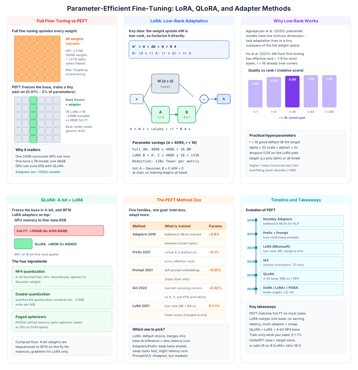
where B has shape (d_out, r) and A has shape (r, d_in). The rank r is a small constant (typically 8-64) independent of the model dimension d. Instead of d_out * d_in trainable parameters, you have r * (d_out + d_in). For d = 4096 and r = 16, that is 131,072 parameters instead of 16,777,216 – a 128x reduction per linear layer.

Anatomy of LoRA

LoRA (Low-Rank Adaptation), introduced by Hu et al. at Microsoft Research in 2021 [3], is the most widely used PEFT method. It adds trainable low-rank matrices to selected linear layers while keeping the base weights frozen.

The Forward Pass

For a linear layer originally computing h = Wx, LoRA changes the computation to:

h = Wx + (alpha / r) * B A x

where:

• W is frozen (pretrained weights, unchanged during fine-tuning)
• A has shape (r, d) initialized from a Gaussian distribution
• B has shape (d, r) initialized to zero
• alpha/r is a scaling factor (alpha is typically set equal to r, making the scale 1.0)

The initial zero initialization of B is critical: at the start of training, B = 0, so dW = B @ A = 0, meaning the model begins as an exact copy of the pretrained base. Training proceeds by computing gradients only for B and A, not for W.

Targeting Specific Layers

In practice, LoRA is typically applied to:

• Query and Value projection matrices in the attention mechanism (W_q and W_v)
• Less commonly, Key and Output projections (W_k and W_o)
• Sometimes the Feed-Forward Network linear layers

Applying LoRA to W_q and W_v is the minimum effective configuration and usually achieves competitive results. Applying it to all four attention projections plus FFN layers increases the trainable parameter count and can improve quality on difficult tasks.

Merging at Inference Time

At deployment time, B and A can be merged into the base weights:

W_merged = W + B @ A

This means the LoRA-adapted model has exactly the same architecture and forward pass as the base model at inference time. There is zero latency overhead compared to full fine-tuning. This is a critical advantage over adapter methods that insert extra layers into the forward pass.

Minimal PyTorch Implementation

Here is a simplified LoRA layer:

import torch
import torch.nn as nn
import torch.nn.functional as F
import math

class LoRALinear(nn.Module):
    """Linear layer with Low-Rank Adaptation."""
    def __init__(self, in_features: int, out_features: int,
                 rank: int = 8, alpha: float = 16.0,
                 dropout: float = 0.05):
        super().__init__()
        # Frozen base weight
        self.base = nn.Linear(in_features, out_features, bias=False)
        self.base.weight.requires_grad = False

        # LoRA parameters
        self.lora_A = nn.Parameter(
            torch.empty(rank, in_features)
        )
        self.lora_B = nn.Parameter(
            torch.zeros(out_features, rank)
        )
        self.scaling = alpha / rank
        self.dropout = nn.Dropout(dropout)

        nn.init.kaiming_uniform_(self.lora_A, a=math.sqrt(5))

    def forward(self, x: torch.Tensor) -> torch.Tensor:
        base_out = self.base(x)
        lora_out = F.linear(self.dropout(x), self.lora_A)
        lora_out = F.linear(lora_out, self.lora_B, scale=self.scaling)
        return base_out + lora_out

    def merge(self):
        self.base.weight.data += (self.lora_B @ self.lora_A) * self.scaling

The implementation shows the key design choices: frozen base, trainable low-rank pair, dropout on the LoRA path, and the merge operation for inference.

Why Low-Rank Works: The Intrinsic Dimension Hypothesis

The idea that pretrained models have low effective dimensionality for downstream tasks was formalized by Aghajanyan et al. (2020) [1]. They showed that for several NLP tasks, the optimal fine-tuning update dW lives approximately in a subspace of dimension 30-200, regardless of the total model size. This means that even a rank-200 decomposition captures nearly all of the task-relevant signal in a weight update that could be millions of parameters wide.

Hu et al. (2021) [3] validated this for transformer fine-tuning: for most layers, the top few singular values of dW dominate the spectrum, and using just 4-16 rank components recovers 95-99% of the fine-tuning quality. A rank of 16 is generally sufficient for most tasks; a rank of 64 is overkill for all but the most demanding applications.

The bar chart in Panel 3 of the diagram illustrates this: quality plateaus rapidly as rank increases beyond 16, with r = 16 already at 99% of the full-rank quality. This is why the “sweet spot” for LoRA is almost always in the range r = 8 to r = 32.

QLoRA: 4-bit Quantization Meets LoRA

If LoRA reduced fine-tuning cost by 100x, QLoRA reduced it by another 10x. Introduced by Dettmers et al. at the University of Washington in 2023 [4], QLoRA combines LoRA with 4-bit quantization of the base weights, enabling fine-tuning of 65B parameter models on a single consumer GPU.

The Memory Problem in LoRA

Even with LoRA, full-precision fine-tuning of large models is expensive because:

• The base model weights W must be loaded into GPU memory in full precision for computation
• Gradients for the LoRA parameters B and A are stored in full precision
• Optimizer states (Adam momentum and variance) for the LoRA parameters also require memory

For a 7B model in FP16, the base weights alone occupy 14GB. For a 65B model, 130GB. This requires multiple GPUs just to hold the model.

QLoRA’s Solution

QLoRA uses four techniques to minimize memory:

1. 4-bit NormalFloat Quantization

NormalFloat (NF4) is a quantization scheme designed specifically for neural network weights [5]. Unlike standard 4-bit quantization (which is optimized for uniform distributions), NF4 uses a quantization grid optimized for Gaussian distributions – which is exactly what pretrained transformer weights follow. NF4 achieves near-lossless compression: a 7B model quantized to NF4 loses only ~0.1% accuracy compared to FP16, while using 4x less memory.

2. Double Quantization

QLoRA quantizes the quantization constants themselves. The NF4 quantization uses a lookup table of 256 values; QLoRA stores this table in 8-bit instead of the original 32-bit. This saves an additional ~0.5GB per 65B model with effectively zero quality loss.

3. Paged Optimizers

Traditional CUDA out-of-memory errors occur when the optimizer state (Adam momentum and variance buffers) exceeds GPU memory. QLoRA uses a paged memory management system inspired by operating system virtual memory: optimizer states that do not fit in GPU memory are spilled to CPU RAM on demand and brought back when needed. This allows fine-tuning models whose optimizer states exceed GPU VRAM without crashing.

4. Dequantize-on-the-Fly

During the forward pass, QLoRA dequantizes only the weights being used for the current matrix multiplication from NF4 to BF16. The computation happens in BF16 (preserving precision), then the result is passed to the next layer. The dequantized weights are discarded after the computation, keeping peak memory low.

What QLoRA Achieves

The results in the QLoRA paper [4] are striking:

Model	Method	GPU Memory	Adapter Quality
7B	Full FT FP16	32GB+	100%
7B	QLoRA NF4	8GB	99%
65B	Full FT FP16	800GB+	100%
65B	QLoRA NF4	48GB	99%
70B	QLoRA NF4	52GB	99%

A single A6000 (48GB) or 2x RTX 3090 (2x24GB) can now fine-tune models that previously required 8x A100s. The quality gap between QLoRA and full FP16 fine-tuning is typically <1 point on standard benchmarks, and in some cases QLoRA actually outperforms full fine-tuning because the 4-bit quantization acts as a regularizer.

Minimal QLoRA Workflow

Here is how you fine-tune a model with QLoRA using the transformers and peft libraries:

import torch
from transformers import AutoModelForCausalLM, AutoTokenizer, BitsAndBytesConfig
from peft import LoraConfig, get_peft_model, TaskType
from datasets import load_dataset

# Step 1: 4-bit quantization config
bnb_config = BitsAndBytesConfig(
    load_in_4bit=True,
    bnb_4bit_quant_type="nf4",
    bnb_4bit_compute_dtype=torch.bfloat16,
    bnb_4bit_use_double_quant=True,
)

# Step 2: Load model quantized to NF4
model = AutoModelForCausalLM.from_pretrained(
    "meta-llama/Llama-2-7b-hf",
    quantization_config=bnb_config,
    device_map="auto",
)

# Step 3: LoRA config
lora_config = LoraConfig(
    task_type=TaskType.CAUSAL_LM,
    r=16,
    lora_alpha=32,
    lora_dropout=0.05,
    target_modules=["q_proj", "v_proj"],
)

# Step 4: Apply LoRA
model = get_peft_model(model, lora_config)
model.print_trainable_parameters()
# trainable params: 4,194,304 || all params: 6,742,609,920 || 0.0622%

# Step 5: Train on your dataset
dataset = load_dataset("your-org/your-dataset")
# ... training loop with Trainer ...

# Step 6: Save adapter (40MB, not 14GB)
model.save_pretrained("./lora-adapter")
tokenizer.save_pretrained("./lora-adapter")

The key point: after training, you save only the adapter weights (a few dozen megabytes), not the full model. You can then combine this adapter with any copy of the base model for inference, or chain multiple adapters for different domains.

The PEFT Method Zoo

LoRA is not the only PEFT method. Several related techniques have been developed, each with different trade-offs:

Houlsby Adapters (2019) [2]

The original adapter-based approach inserts a small bottleneck MLP (multi-layer perceptron) after each attention and FFN sublayer. Each adapter consists of a down-projection to a small hidden dimension (typically 64-256), a non-linearity, and an up-projection back to the original dimension. The adapter adds parameters in series rather than parallel, meaning the forward pass is extended:

h = LayerNorm(x + Attention(x) + Adapter_1(x))
h = LayerNorm(h + FFN(h) + Adapter_2(h))

Adapters typically add ~3.6% overhead to the parameter count and introduce a small latency penalty (the extra matrix multiplication). They have largely been superseded by LoRA for most use cases.

Prefix Tuning (2021) [6]

Prefix tuning prepends a sequence of learnable vectors to the Key and Value tensors at every attention layer. These “virtual tokens” provide context that the model attends to, allowing task-specific behavior without modifying any weights. The trainable parameters are the prefix vectors (typically 512 tokens x 4096 dimensions per layer), which is ~0.1% of the total parameter count.

Prefix tuning is effective for generation tasks (summarization, dialogue) but less so for discriminative tasks (classification, extraction). The inference cost is slightly higher because the prefix tokens are attended to at every layer.

Prompt Tuning (2021) [7]

Prompt tuning is a simplification of prefix tuning: instead of prepending prefixes at every attention layer, it prepends learnable embedding vectors only at the input layer. The model’s own attention mechanism propagates these task-specific prompts through the network. The trainable parameter count is the smallest of any PEFT method (~0.01%) but the quality is also the weakest, especially for large models or difficult tasks.

IA3 (2022) [8]

IA3 (Infused Adapter by Inhibiting and Amplifying Inner Activations) introduces learned vectors that rescale element-wise the Key, Value, and FFN intermediate activations. The idea is that task adaptation can be expressed as amplifying or attenuating existing activation channels rather than adding new transformations:

h = (l_v * V(x)) @ softmax((l_q * Q(x)) @ (l_k * K(x))^T / sqrt(d))

where l_q, l_k, l_v are trainable vectors of shape (d,). IA3 has extremely few trainable parameters (~0.02%) and surprisingly strong performance on certain tasks. It won the BigBench Hard Leaderboard in 2022 using the T5-XXL model.

Method Comparison

Method	What is Trained	Relative Params	Inference Overhead
Full FT	All weights	100%	None
Houlsby Adapters	Bottleneck MLPs at every layer	~3.6%	Small (extra MLP per layer)
Prefix Tuning	Virtual K,V tokens at every attention layer	~0.1%	Small (extra token attention)
Prompt Tuning	Input-level soft prompt embeddings	~0.01%	None (single embedding lookup)
IA3	Rescaling vectors on K, V, FFN	~0.02%	None (element-wise multiply)
LoRA	Low-rank B,A on selected linear layers	0.1-1%	None (merged into base)
QLoRA	LoRA + 4-bit NF4 base	0.1-1%	None (merged, base is 4-bit)

LoRA’s key advantage over all competing methods is its zero-inference-cost design. The merge step produces an exact copy of the base model with the full-rank update baked in, so serving a LoRA-adapted model has identical latency and memory to serving the base model.

Multi-Adapter Serving

Because LoRA adapters are small (typically 10-100MB) and can be merged into the base model at inference time, you can serve a single base model with multiple task-specific adapters. A 70B base model in FP16 occupies ~140GB of VRAM. A separate 70B fine-tuned copy for each task would require 140GB per task. With LoRA, you store one 140GB base plus a few hundred MB of adapters for each task.

Frameworks like vLLM and Text Generation Inference (TGI) now support dynamic adapter loading: you can swap between adapters without restarting the server, and even batch requests from different tasks together on the same GPU. This makes LoRA the backbone of multi-task LLM serving architectures.

Hyperparameter Guide

Getting LoRA right is mostly about choosing the target modules, rank, and learning rate:

Rank (r):

• r = 8-16: Good default for most tasks; trains quickly, adapters are small
• r = 32-64: Useful for complex tasks with large datasets (>100K examples)
• r = 128+: Only for the hardest tasks; may overfit on small datasets

Alpha and Scale:

• alpha = r gives alpha/r = 1.0, which is the most common setting
• Some practitioners set alpha = 2 * r to make the LoRA contribution larger during early training

Target Modules:

• ["q_proj", "v_proj"]: Minimum effective; ~0.05% of model parameters
• ["q_proj", "k_proj", "v_proj", "o_proj"]: Full attention; ~0.1%
• ["q_proj", "k_proj", "v_proj", "o_proj", "gate_proj", "up_proj", "down_proj"]: Full attention + FFN; ~0.3-1%

Dropout:

• 0.05 is the standard choice; helps prevent overfitting on small datasets
• Can be reduced to 0.01 or 0 for very large datasets

Learning Rate:

• 1e-4 to 5e-4 is typical for the LoRA parameters
• The base model learning rate is effectively 0 (frozen)

Recent Advances

Several improvements to LoRA have been proposed since 2021:

DoRA (Weight-Decomposed Low-Rank Adaptation, 2024) [9]: DoRA decomposes the weight matrix into magnitude and direction components, training only the direction via LoRA while normalizing the magnitude. This improves training stability and can achieve better quality than standard LoRA for the same rank.

LoRA+ (2024) [10]: LoRA+ applies different learning rates to the B and A matrices, using a 16:1 ratio (B gets the higher LR). This addresses the asymmetry in initialization: B starts at zero (needs more LR to learn) while A starts from Gaussian (converges faster).

PiSSA (Principal Singular Value Adaptation, 2024) [11]: Instead of initializing B to zero and A to Gaussian, PiSSA initializes the LoRA parameters using the principal singular vectors of the pretrained weight matrix. This makes fine-tuning start closer to the pretrained optimum, leading to faster convergence and better final quality.

When to Use PEFT (and When Not To)

PEFT is the default choice when:

• You need to adapt a large model to a specific domain or task
• You have limited GPU resources (single GPU or small cluster)
• You want to serve multiple task variants from one base model
• You need fast iteration on multiple fine-tuning experiments

Full fine-tuning may still be preferable when:

• You have sufficient compute and need maximum quality on a single task
• You are training a model from scratch (no pretrained base exists)
• The task requires fundamentally new capabilities not present in the base model
• You need the model to forget or unlearn specific knowledge

Practical Takeaways

1. LoRA is the default. It achieves quality competitive with full fine-tuning at 100x lower cost and zero inference overhead. Unless you have a specific reason to use another method, use LoRA.

2. QLoRA makes large-model fine-tuning accessible. With 4-bit NF4 quantization, models up to 70B parameters can be fine-tuned on consumer hardware. This has democratized model adaptation.

3. Rank is cheap but not free. r = 16 is almost always sufficient. Going higher than r = 64 rarely improves quality and increases both training time and adapter size.

4. Target more layers for hard tasks. For domain adaptation with large datasets (>100K examples), applying LoRA to all attention projections plus FFN layers (not just Q and V) gives better results.

5. Adapters are portable and composable. You can stack multiple LoRA adapters (e.g., one for domain adaptation, one for instruction tuning) and merge them sequentially or simultaneously.

6. The ecosystem is mature. Hugging Face PEFT, vLLM, TGI, and Unsloth all support LoRA/QLoRA out of the box. Training a LoRA model in 2026 is a matter of configuring the right hyperparameters, not implementing algorithms from scratch.

Summary

Parameter-Efficient Fine-Tuning has transformed how we adapt large language models. LoRA’s insight – that task-specific weight updates live in low-dimensional subspaces – enabled training 0.1% of a model’s parameters while preserving 99% of its quality. QLoRA combined this with 4-bit quantization to bring 65B-model fine-tuning to a single consumer GPU. The PEFT ecosystem has matured into a reliable, well-supported stack with multiple methods for different trade-off profiles.

For anyone working with LLMs in 2026, understanding PEFT is not optional. It is the practical answer to “how do I customize this powerful model to my domain without a supercomputer?” and the foundation of modern multi-task LLM serving architectures.

References

[1] Aghajanyan, A. et al. “Intrinsic Dimensionality Explains the Effectiveness of Language Model Fine-Tuning.” ACL 2021. arXiv:2012.13255

[2] Houlsby, N. et al. “Parameter-Efficient Transfer Learning for NLP.” ICML 2019. arXiv:1902.00751

[3] Hu, E.J. et al. “LoRA: Low-Rank Adaptation of Large Language Models.” ICLR 2022. arXiv:2106.09685

[4] Dettmers, T. et al. “QLoRA: Efficient Finetuning of Quantized LLMs.” ACL 2024. arXiv:2305.14314

[5] Dettmers, T. et al. “LLM.int8(): 8-bit Matrix Multiplication for Transformers at the Scale of 100 Billions of Parameters.” ICLR 2023. arXiv:2208.07339

[6] Li, X.L., Liang, P. “Prefix-Tuning: Optimizing Continuous Prompts for Generation.” ACL 2021. arXiv:2101.00190

[7] Lester, B., Al-Rfou, R., Constant, N. “The Power of Scale for Parameter-Efficient Prompt Tuning.” EMNLP 2021. arXiv:2104.08691

[8] Liu, H. et al. “IA3: Infused Adapter by Inhibiting and Amplifying Inner Activations.” ICML 2022. arXiv:2205.05638

[9] Liu, S.Y. et al. “DoRA: Weight-Decomposed Low-Rank Adaptation.” ICML 2024. arXiv:2402.09353

[10] Hayou, S. et al. “LoRA+: Efficient Low Rank Adaptation of Large Models.” ICML 2024. arXiv:2402.12354

[11] Meng, F. et al. “PiSSA: Principal Singular Values and Singular Vectors Adaptation of Large Language Models.” NeurIPS 2024. arXiv:2404.02948

Enjoyed this post? Never miss out on future posts by following us