I Built an LLM From Scratch: 30M Parameters, 4 Hours, 1 GPU

There is a particular kind of understanding that only comes from building the thing yourself. I have written about tokenizers, attention, KV-caches, and sampling in this series – but writing about components is not the same as watching a matrix of random numbers slowly learn to tell stories. So I built a small GPT from scratch in plain PyTorch: 30 million parameters, trained on children’s stories for about four hours on a single RTX 4090, for roughly two dollars of electricity. No Trainer class, no Lightning, no configuration files – about 600 lines of code where every tensor operation is mine. This post is the honest account of what happened, what broke, and what I learned.

This is the eighth post in our LLM internals series, and it ties the previous seven together: tokenization, attention, KV-cache, inference phases, the training pipeline, quantization, and sampling strategies.

The Journey at a Glance

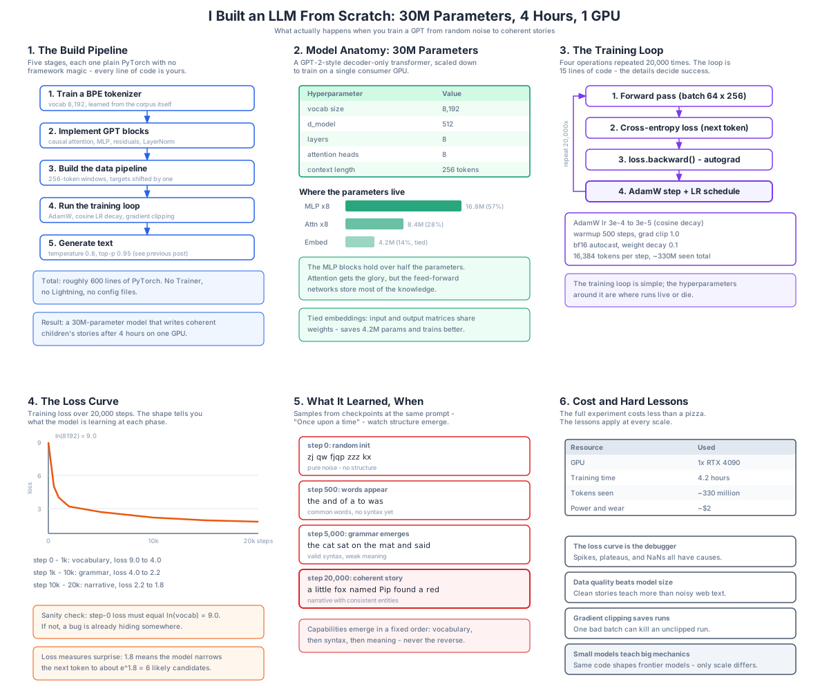
Understanding the Diagram

The diagram breaks the project into six panels: the build pipeline, the model anatomy, the training loop, the loss curve, the learning progression, and the true cost.

Panel 1: The Build Pipeline

The top-left panel shows the five stages in order. First, train a BPE tokenizer on the corpus itself – I used a vocabulary of 8,192, far smaller than GPT-2’s 50,257, because a children’s-story vocabulary is tiny and a small vocab shrinks the embedding table. Second, implement the GPT blocks: causal multi-head attention, feed-forward networks, residual connections, and LayerNorm. Third, build the data pipeline that slices tokenized text into 256-token windows with targets shifted by one position. Fourth, run the training loop. Fifth, generate text with the sampling strategies from the previous post. The whole thing is about 600 lines of PyTorch, and the result is a model that writes coherent stories after four hours.

Panel 2: Model Anatomy

The top-middle panel shows where the 30 million parameters live. The configuration is deliberately modest: 8 layers, 8 heads, d_model of 512, context of 256 tokens. The surprise for most people is the distribution: the MLP blocks hold 57% of all parameters (16.8M), attention holds only 28% (8.4M), and the tied embedding matrix holds the remaining 14%. Attention gets the glory in explanations of transformers, but the feed-forward networks store most of the model’s knowledge. Tying the input embedding and output projection matrices saves 4.2M parameters and measurably trains better.

Panel 3: The Training Loop

The top-right panel shows the loop itself: forward pass on a batch of 64 by 256 tokens, cross-entropy loss on next-token prediction, loss.backward(), and an AdamW step with a learning-rate schedule – repeated 20,000 times. The loop body is about 15 lines. The details around it decide whether the run lives or dies: warmup of 500 steps, cosine decay from 3e-4 to 3e-5, gradient clipping at 1.0, bf16 autocast, weight decay 0.1. Each of those settings exists because a run failed without it.

Panel 4: The Loss Curve

The bottom-left panel plots training loss across the 20,000 steps, and its shape tells you what the model is learning. The first sanity check happens at step 0: with random weights, the model is uniform over the vocabulary, so the loss must equal ln(8,192) = 9.0. If your step-0 loss is anything else, a bug is already hiding somewhere. The curve then drops fast to about 4.0 in the first thousand steps (the model learns vocabulary), grinds slowly from 4.0 to 2.2 (grammar), and flattens toward 1.8 (narrative structure). A loss of 1.8 means the model has narrowed the next token down to roughly e^1.8 – about six likely candidates – at every position.

Panel 5: What It Learned, When

The bottom-middle panel shows generations from saved checkpoints, all given the prompt “Once upon a time”. At step 0 the output is noise: “zj qw fjqp zzz kx”. At step 500, common words appear without syntax: “the and of a to was”. At step 5,000, grammar emerges: “the cat sat on the mat and said”. At step 20,000, the model tells a story with consistent entities: “a little fox named Pip found a red…”. Capabilities always emerged in the same order – vocabulary, then syntax, then meaning. Never the reverse.

Panel 6: Cost and Hard Lessons

The bottom-right panel totals the bill: one RTX 4090, 4.2 hours, about 330 million tokens seen, roughly two dollars of power and wear. The lessons cost more than the money: the loss curve is your debugger, data quality beats model size, gradient clipping saves runs, and small models teach the same mechanics as frontier ones – only the scale differs.

Stage 1: The Tokenizer

Everything in the tokenization post became real the moment I trained my own BPE tokenizer. The corpus is TinyStories – a synthetic dataset of short children’s stories generated by GPT-3.5/4, designed so that small models can actually learn grammar and narrative. Training BPE on it with a target vocabulary of 8,192 took minutes, and the resulting merges were a delight to inspect: “once”, “upon”, “little”, and “ mommy” (with the leading space) were among the first merges learned.

Two decisions mattered here. First, a small vocabulary: TinyStories uses simple English, so 8,192 tokens covers it well, and the embedding table shrinks to 4.2M parameters instead of the 25.7M that GPT-2’s vocabulary would cost. Second, training the tokenizer on the same corpus as the model: an off-the-shelf tokenizer wastes hundreds of vocabulary slots on tokens the corpus never uses.

Stage 2: The Model

The model is a GPT-2-style decoder-only transformer, small enough to train quickly but complete enough that every mechanism from the attention post is present. The core block is about 50 lines:

import torch
import torch.nn as nn
import torch.nn.functional as F

class Block(nn.Module):
    def __init__(self, d_model=512, n_head=8):
        super().__init__()
        self.ln1 = nn.LayerNorm(d_model)
        self.attn = nn.MultiheadAttention(d_model, n_head, batch_first=True)
        self.ln2 = nn.LayerNorm(d_model)
        self.mlp = nn.Sequential(
            nn.Linear(d_model, 4 * d_model),
            nn.GELU(),
            nn.Linear(4 * d_model, d_model),
        )

    def forward(self, x, mask):
        h = self.ln1(x)
        a, _ = self.attn(h, h, h, attn_mask=mask, need_weights=False)
        x = x + a                       # residual connection
        x = x + self.mlp(self.ln2(x))   # residual connection
        return x

The full model stacks eight of these blocks between a token-plus-position embedding and a final LayerNorm with a tied output projection. Two implementation details bit me. First, the causal mask: nn.MultiheadAttention expects a boolean mask where True means “blocked”, so the mask is an upper-triangular matrix of True above the diagonal – getting this backwards lets the model cheat by looking at the future, and the loss drops suspiciously fast before you notice. Second, initialization: PyTorch’s defaults work, but scaling the residual-path projections down by 1/sqrt(2 * n_layer) (as GPT-2 does) noticeably stabilized the early loss curve.

Stage 3: The Data Pipeline

The data pipeline tokenizes the entire corpus once, concatenates it into a single token stream, and slices out random 256-token windows at every training step. The target sequence is the input sequence shifted by one position – the model learns to predict token t+1 from tokens 0..t at every position in parallel. That shift is the entire “dataset engineering” of GPT pretraining:

def get_batch(tokens, batch_size=64, ctx=256, device="cuda"):
    ix = torch.randint(0, len(tokens) - ctx - 1, (batch_size,))
    x = torch.stack([tokens[i : i + ctx] for i in ix]).to(device)
    y = torch.stack([tokens[i + 1 : i + ctx + 1] for i in ix]).to(device)
    return x, y

With 64 sequences of 256 tokens per step, every optimizer step sees 16,384 tokens. Over 20,000 steps the model consumed about 330 million tokens – several passes over the TinyStories training split.

Stage 4: The Training Loop

The loop is the least glamorous and most instructive part:

model = GPT(vocab_size=8192, d_model=512, n_layer=8, n_head=8, ctx=256).cuda()
opt = torch.optim.AdamW(model.parameters(), lr=3e-4, weight_decay=0.1)

for step in range(20_000):
    x, y = get_batch(train_tokens)
    lr = cosine_lr(step, base=3e-4, final=3e-5, warmup=500, total=20_000)
    for g in opt.param_groups:
        g["lr"] = lr

    with torch.autocast("cuda", dtype=torch.bfloat16):
        logits = model(x)
        loss = F.cross_entropy(logits.view(-1, 8192), y.view(-1))

    opt.zero_grad(set_to_none=True)
    loss.backward()
    torch.nn.utils.clip_grad_norm_(model.parameters(), 1.0)
    opt.step()

    if step % 500 == 0:
        print(f"step {step:6d}  loss {loss.item():.4f}  lr {lr:.2e}")

Every line earned its place. The warmup prevents early loss explosions when the AdamW second-moment estimates are garbage. Gradient clipping saved the run twice – around step 12,000 a single bad batch spiked the gradient norm to 40, and without clipping that one step would have poisoned the weights. bf16 autocast doubled throughput on the 4090 with zero visible effect on the loss curve. The cosine decay to a small nonzero floor produced the classic late-training improvement in the final 2,000 steps.

Stage 5: Generation

Generation reuses exactly the machinery from the sampling post: forward pass, take the logits of the last position, divide by temperature, truncate with top-p, sample, append, repeat. At this scale there is no need for a KV-cache – a 256-token context recomputes in milliseconds – but adding one later is a satisfying exercise from the KV-cache post.

The checkpoint samples were the emotional payoff of the whole project. Watching “zj qw fjqp” become “the and of a to” become “the cat sat on the mat” become an actual story about a fox named Pip – that progression, more than any paper, is what taught me what pretraining actually does. The model never sees a labeled example of grammar. Syntax emerges purely because predicting the next token is easier when you know how sentences work.

What It Actually Cost

Resource	Used
GPU	1x RTX 4090 (24 GB)
Training time	4.2 hours
Tokens seen	~330 million
Power and wear	~$2
Lines of code	~600

The contrast with frontier training is the point: GPT-3 cost an estimated $4.6M in compute. My model is 6,000 times smaller and speaks only in children’s stories, but every mechanism – embeddings, attention, residuals, layernorm, AdamW, cosine schedules, sampling – is the same machinery. Scale adds capability; it does not add new principles.

Lessons Learned

The loss curve is the debugger. A plateau at 3.5 means something different from a plateau at 2.0. A sudden spike means a bad batch or an LR problem. A NaN after step 10,000 usually means missing gradient clipping. You learn to read the curve the way a mechanic learns to listen to an engine.

Data quality beats model size. TinyStories is synthetic, clean, and narrow – and that is exactly why a 30M model can master it. Doubling the model on noisy web text would have produced a worse result for more money.

Gradient clipping is not optional. It is two lines of code and it saved the run twice. Every untrained urge to skip it should be resisted.

Sanity checks catch bugs early. The ln(vocab) check at step 0, overfitting a single batch to near-zero loss, and generating text every 500 steps caught three separate bugs in one afternoon.

Small models teach big mechanics. Everything in this series – the attention math, the KV-cache tradeoff, the quantization formats, the sampling knobs – exists in this 600-line program. If you want to understand LLMs, building one at this scale is the highest-value weekend you can spend.

Related Posts

• LLM Tokenization: How Text Becomes Numbers
• LLM Attention Mechanism: The Heart of the Transformer
• LLM Decode: KV-Cache and GPU VRAM Deep Dive
• LLM Prompt vs Decode: Understanding the Two Phases of Inference
• LLM Training Pipeline: From Pretraining to RLHF and DPO
• LLM Quantization: Running 70B Models on a Laptop with FP16, INT8, and INT4
• LLM Sampling and Decoding Strategies: Temperature, Top-k, Top-p, Min-p, and Beam Search

Further Reading

• nanoGPT by Andrej Karpathy – the cleanest minimal GPT training implementation
• TinyStories dataset – the corpus used for this build
• Attention Is All You Need (paper) – the original transformer architecture

Conclusion

Building an LLM from scratch is not about competing with anyone’s model. A 30M-parameter GPT trained on children’s stories will never answer your emails. What it gives you is something no amount of reading can: the moment a loss curve bends and random weights become grammar, you stop thinking of LLMs as magic and start thinking of them as machines. Every post in this series describes one component of that machine – but assembling all of them with your own hands is what makes the understanding permanent. If you have a GPU and a free afternoon, take the 600 lines and run them. The fox named Pip is waiting.

Enjoyed this post? Never miss out on future posts by following us