LLM Tokenization: How Text Becomes Numbers

Large language models do not read text. They process sequences of integers. Before a single token of your prompt reaches the transformer layers, it must pass through a tokenizer – a deterministic algorithm that chops raw text into discrete units called tokens and maps each one to a unique integer ID. This process, called tokenization, is the invisible bridge between human language and machine computation.

Despite being the very first step in the LLM pipeline, tokenization is poorly understood by most practitioners. It affects everything from API costs to context window limits, from multilingual performance to code generation quality. In this post, we will trace the complete journey from raw text to embedding vectors, explain the Byte-Pair Encoding (BPE) algorithm that powers most modern tokenizers, and show why tokenization choices have outsized practical consequences.

This is the third post in our LLM internals series, following LLM Prompt vs Decode and KV-Cache and GPU VRAM Deep Dive.

The Tokenization Pipeline

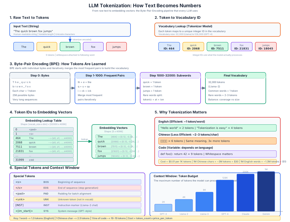
Understanding the Diagram

The diagram above traces the complete tokenization pipeline through six interconnected sections. Let us examine each in detail.

Section 1: Raw Text to Tokens

The process begins with a raw string – human-readable text composed of Unicode characters. The input “The quick brown fox jumps” enters the tokenizer, which splits it into five discrete token units. Note a critical detail: whitespace is typically attached to the following word rather than being a standalone token. The token “ quick” includes the leading space. This is not arbitrary – it reduces the total number of tokens by combining the space with the word, and it preserves the information needed to reconstruct the original text.

The tokenizer does not simply split on word boundaries. Punctuation, contractions, numbers, and code all follow language-specific rules. The word “don’t” might become [“don”, “‘t”] or [“do”, “n’t”] depending on the tokenizer. The string “3.14159” might be one token or several, depending on whether the tokenizer learned to merge digit sequences during training.

Section 2: Token to Vocabulary ID

Once the text is split into tokens, each token is looked up in a fixed vocabulary table that maps strings to integer IDs. The vocabulary is learned during tokenizer training (before model training begins) and never changes during inference. “The” maps to ID 464, “ quick” to ID 2068, “ brown” to ID 7511, and so on.

These integer IDs are what the model actually processes. The transformer never sees the string “fox” – it sees the integer 21831. The vocabulary size is a critical design decision: Llama-2 uses 32,000 tokens, GPT-4 uses approximately 128,000, and Llama-3 uses 128,256. A larger vocabulary means more tokens are represented as single units (reducing sequence length) but also means the embedding table is larger (increasing memory usage).

Section 3: Byte-Pair Encoding (BPE)

BPE is the algorithm that builds the vocabulary. It was originally a data compression technique and was adapted for NLP by Sennrich et al. in 2015. The algorithm works in four stages:

Stage 0 – Bytes: Start with the 256 possible byte values as the initial vocabulary. Every character is represented as a single byte. At this stage, the word “the” requires 3 tokens (t, h, e), and a long text produces a very long token sequence.

Stage 1-1000 – Frequent Pairs: Count all adjacent token pairs across the training corpus. Find the most frequent pair (e.g., “t” + “h” appears millions of times) and merge them into a new token “th”. Repeat this process: next, “th” + “e” might merge into “the”. Each merge adds one new token to the vocabulary.

Stage 1000-32000 – Subwords: After thousands of merges, common words like “quick”, “brown”, and “jumps” have been merged into single tokens. Rare words that did not appear frequently enough in the training data remain split into subword units. For example, “tokenization” might become [“token”, “iz”, “ation”] – three tokens that together cover the word without needing a dedicated vocabulary entry.

Final Vocabulary: The process stops when the target vocabulary size is reached (e.g., 32,000 for Llama-2). The resulting vocabulary contains: individual bytes (for fallback), common subwords, and frequent whole words. This design means the tokenizer can represent ANY text – even words it has never seen before – as a sequence of subword tokens, without ever producing an “unknown” token.

Section 4: Token IDs to Embedding Vectors

After tokenization, the integer IDs are converted to dense vectors through an embedding lookup. The embedding table is a matrix of shape [vocab_size x dim] – for Llama-2 7B, this is [32000 x 4096], occupying approximately 250 MB in FP16. Each row of this matrix is the learned vector representation of one token.

The lookup is a simple indexing operation: token ID 464 retrieves row 464 from the embedding matrix, producing a 4096-dimensional vector. These vectors are learned during model training – they are not random. Tokens with similar meanings tend to have similar embeddings because the model learns to place them near each other in vector space.

The output of this step is a sequence of embedding vectors – one per input token – that then flows through the transformer layers (self-attention, feed-forward networks, layer normalization) to produce the final output.

Section 5: Why Tokenization Matters

Tokenization efficiency varies dramatically across languages and content types:

English (Efficient): English text averages approximately 1.3 tokens per word because the tokenizer has been trained predominantly on English data. “Hello world” = 2 tokens. “Tokenization is easy” = 4 tokens. This efficiency means English prompts are cheaper and fit more content within the context window.

Chinese (Less Efficient): Chinese characters typically require 2-3 tokens each because Chinese text was less common in the training corpus. The same meaning “Hello world” in Chinese requires 6 tokens – 3x more than English. This has real cost implications: processing 1 million Chinese characters costs approximately 3x more than 1 million English words.

Code (Variable): Programming code is tokenized inconsistently. “def foo(): return 42” becomes approximately 9 tokens. Whitespace indentation in Python is tokenized separately, meaning deeply nested code consumes more tokens. This is why code-heavy prompts can quickly consume context window budget.

Section 6: Special Tokens and Context Window

Special tokens are non-text tokens reserved for structural purposes. They are inserted by the model’s chat template, not by the user:

• BOS (Beginning of Sequence): Marks the start of input
• EOS (End of Sequence): Signals the model to stop generating
• PAD (Padding): Fills batches when sequences have different lengths
• UNK (Unknown): Fallback for tokens not in vocabulary (rare with BPE)
• [INST]: Llama-2’s instruction marker for chat formatting

• **<

  im_start

  >**: GPT-style system message marker

The context window is the maximum number of tokens the model can process in a single request, including both input (prompt) and output (generated text). The diagram shows how context windows have grown exponentially: from GPT-3’s 2K tokens (2020) to Gemini 1.5 Pro’s 1M tokens (2024). Each 4x increase in context window roughly doubles the KV-cache memory requirement (as explained in our KV-cache deep dive).

How BPE Actually Works: A Worked Example

Let us trace through a simplified BPE training process. Suppose our training corpus contains:

low (5x)    lower (2x)    newest (6x)    widest (3x)

Step 0: Initialize vocabulary with characters. Each word is split into characters plus an end-of-word marker:

l o w </w>  (5x)
l o w e r </w>  (2x)
n e w e s t </w>  (6x)
w i d e s t </w>  (3x)

Step 1: Count all adjacent pairs. The pair (e, s) appears in “newest” (6x) and “widest” (3x) = 9 total. This is the most frequent pair. Merge:

l o w </w>  (5x)
l o w e r </w>  (2x)
n e w es t </w>  (6x)
w i d es t </w>  (3x)

Step 2: Next most frequent pair is (es, t) appearing 9 times. Merge:

l o w </w>  (5x)
l o w e r </w>  (2x)
n e w est </w>  (6x)
w i d est </w>  (3x)

Step 3: The pair (l, o) appears 7 times (5x in “low” + 2x in “lower”). Merge:

lo w </w>  (5x)
lo w e r </w>  (2x)
n e w est </w>  (6x)
w i d est </w>  (3x)

Step 4: The pair (lo, w) appears 7 times. Merge:

low </w>  (5x)
low e r </w>  (2x)
n e w est </w>  (6x)
w i d est </w>  (3x)

After 4 merges, “low” is now a single token. If we continue, eventually “newest” and “widest” will become single tokens, and the vocabulary will contain both common words and subword fragments.

At inference time, the tokenizer applies the learned merges in order. The word “lower” (not in the training data as a whole) would be tokenized as [“low”, “er”] – two subword tokens that together cover the word.

Tokenizer Variants: BPE vs WordPiece vs SentencePiece

While BPE is the most common algorithm, there are important variants:

Byte-Level BPE (used by GPT-4, Llama-3): Instead of operating on Unicode characters, it operates on raw bytes. This guarantees that any text can be tokenized without an UNK token, because there are only 256 possible bytes and they cover all possible inputs. GPT-4’s tokenizer (cl100k_base) and Llama-3’s tokenizer both use byte-level BPE.

WordPiece (used by BERT): Similar to BPE but uses a different merge criterion. Instead of merging the most frequent pair, WordPiece merges the pair that maximizes the likelihood of the training data. This tends to produce slightly different subword boundaries.

SentencePiece (used by Llama-2, T5): A library that implements BPE or Unigram tokenization but treats the input as a raw byte stream – no pre-tokenization into words. This means it does not need whitespace to delimit tokens and can handle languages without word boundaries (Chinese, Japanese, Thai) more naturally. Llama-2 uses SentencePiece with BPE.

Unigram (used by T5, ALBERT): Starts with a large vocabulary and iteratively removes tokens that contribute least to the likelihood of the training data. This produces a probabilistic tokenizer where a given text can have multiple valid tokenizations, and the one with the highest probability is chosen.

Practical Implications

API Costs: All major LLM APIs (OpenAI, Anthropic, Google) charge per token, not per character or word. Understanding tokenization helps you estimate costs:

• 1 English word ~= 1.3 tokens
• 1 Chinese character ~= 2.5 tokens
• 1 line of Python code ~= 10-15 tokens
• 1 page of text (~500 words) ~= 650 tokens

At GPT-4’s pricing of $0.01 per 1K input tokens, processing a 100-page document (65,000 tokens) costs $0.65 per request. If the document is in Chinese, the cost triples to ~$2.00.

Context Window Budget: Every token in your prompt counts against the context window. A 4K-token context window holds approximately 3,000 English words or ~1,500 Chinese characters. Knowing your tokenizer helps you maximize the useful content within the budget. Use len(tokenizer.encode(text)) to check token counts before sending requests.

Multilingual Performance: Models with tokenizers trained predominantly on English (like early GPT models) are less efficient and sometimes less capable in other languages. The higher token count for non-English text means less context fits in the window, and the model has less “room” to reason. Models like Llama-3 (128K vocab) and Qwen (152K vocab) explicitly expanded their vocabulary to include more non-English tokens, improving both efficiency and quality.

Code Generation: Code tokenization is particularly tricky. Python’s significant whitespace means indentation tokens are critical. Some tokenizers handle this well (GPT-4), while others waste tokens on repeated whitespace. If you are building a coding assistant, test your tokenizer on representative code snippets to understand the token overhead.

Prompt Engineering: Certain words and phrases are more token-efficient than others. “However” is one token in most tokenizers, while “nevertheless” might be two or three. When optimizing prompts for cost or context window, replacing verbose phrases with concise alternatives that happen to be single tokens can save meaningful budget.

Tokenization Tools

You can experiment with tokenization using these open-source libraries:

• tiktoken: OpenAI’s fast BPE tokenizer (Rust + Python). Supports GPT-3.5 and GPT-4 tokenizers. Use tiktoken.encoding_for_model("gpt-4") to get the correct tokenizer.
• SentencePiece: Google’s tokenizer library supporting BPE and Unigram. Used by Llama-2, T5, and many other models.
• Hugging Face tokenizers: Rust-based library supporting BPE, WordPiece, and Unigram with a Python interface. Works with any model on the Hub.

Further Reading

• Neural Machine Translation of Rare Words with Subword Units (Sennrich et al., 2015) – The paper that introduced BPE for NLP
• Attention Is All You Need (Vaswani et al., 2017) – The Transformer paper that uses token embeddings as input

Related Posts

• LLM Prompt vs Decode: Understanding the Two Phases of LLM Inference
• LLM Decode Deep Dive: KV-Cache, GPU VRAM, and the Memory Bottleneck
• AI Coding FAQ: 20 Most Asked Questions

Conclusion

Tokenization is the first and most fundamental step in the LLM pipeline. It determines how much text fits in your context window, how much you pay per API call, and how well the model handles different languages. BPE – the dominant algorithm – elegantly balances vocabulary size with coverage by starting from individual bytes and iteratively merging the most frequent pairs.

The key takeaways are: (1) tokens are not words – they are subword units whose boundaries are determined by the tokenizer’s training data; (2) tokenization efficiency varies by language, with English being the most efficient and non-Latin scripts being 2-3x more expensive; (3) the vocabulary size is a design tradeoff between sequence length and embedding table memory; (4) context windows are measured in tokens, not characters, so tokenizer efficiency directly determines how much content you can process.

Understanding tokenization is not just academic – it is the foundation for cost optimization, context window management, and multilingual model selection. Every token saved is real money saved and real context budget preserved.

Enjoyed this post? Never miss out on future posts by following us