LLM Decode Deep Dive: KV-Cache, GPU VRAM, and the Memory Bottleneck

In the previous post, we established that LLM inference has two phases: prompt (prefill) and decode. We learned that prefill is compute-bound while decode is memory-bandwidth-bound. But we did not answer the deeper question: what exactly lives in GPU VRAM during decode, and why does it create a bottleneck?

This post goes under the hood. We will dissect the KV-cache, map it to physical GPU VRAM, trace the exact memory reads and writes that happen during each decode step, and explain why adding more GPU compute power does not make decoding faster. We will also cover the three major optimization techniques – PagedAttention, FlashAttention, and KV cache quantization – that production systems use to mitigate this bottleneck.

What Is the KV-Cache?

The KV-cache is a memory buffer that stores intermediate computation results from the transformer’s self-attention layers. Specifically, it stores the Key (K) and Value (V) tensors for every token that has been processed so far – both the prompt tokens and all generated output tokens.

Without the KV-cache, generating the Nth output token would require recomputing the K and V tensors for all N-1 previous tokens from scratch. For a 1,000-token output, that means recomputing 999 tokens’ attention values 1,000 times – a quadratic cost that makes autoregressive generation impractically slow.

The KV-cache eliminates this redundancy. Once a token’s K and V tensors are computed, they are stored in the cache and reused for every subsequent token. This reduces the per-token cost from O(N) to O(1) in terms of computation – but at the cost of O(N) memory storage that must be read every step.

The KV-Cache Formula

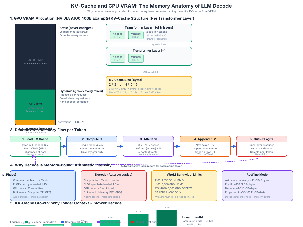
Understanding the Diagram

The diagram above provides a comprehensive view of how the KV-cache interacts with GPU VRAM during the decode phase. Let us examine each section in detail.

Section 1: GPU VRAM Allocation

The left section shows the physical memory layout of an NVIDIA A100 40GB GPU when serving a 13B parameter model. VRAM is divided into three categories:

Model Weights (26 GB, 65%) The model’s parameters are loaded into VRAM once at startup and never change. For a 13B parameter model in FP16 (2 bytes per parameter), this consumes 26 GB. This memory is static – it persists for the entire lifetime of the server and is shared across all concurrent requests. The model weights are read during every forward pass (both prefill and decode), but they are never written to.

KV-Cache (12 GB, 30%) This is the dynamic portion that grows and shrinks with each request. When a new request arrives, the prefill phase populates the KV-cache with all prompt tokens’ K,V values. During decode, each new token’s K,V values are appended. When the request completes, its KV-cache is freed. The 12 GB shown here is a snapshot – in practice, the KV-cache budget is configured as a fraction of total VRAM (typically 30-40%) and determines how many concurrent requests the server can handle.

Activations (2 GB, 5%) Temporary tensors created during the forward pass – intermediate attention scores, FFN outputs, softmax results. These are allocated, used, and freed within a single forward pass. Their size depends on batch size and sequence length but is generally small compared to weights and KV-cache.

The critical insight is that only the KV-cache portion is dynamic. Model weights and activation budgets are predictable, but KV-cache usage depends on the length of each conversation – which is unknown until the request completes. This unpredictability is the root cause of memory management challenges in LLM serving.

Section 2: KV-Cache Structure

The right-top section shows the internal structure of the KV-cache. For each transformer layer, there are separate K and V tensors, each with dimensions [num_heads x head_dim x seq_len]. The total KV-cache size follows this formula:

KV_cache_bytes = 2 (K+V) x 2 (FP16) x num_layers x num_heads x head_dim x seq_len

For Llama-2 7B (32 layers, 32 heads, 128 dim): each token requires 2 x 2 x 32 x 32 x 128 = 524,288 bytes = 0.5 MB. A 4,000-token context therefore needs 2 GB of KV-cache. A 32,000-token context needs 16 GB – nearly half the A100’s total VRAM.

The cache is replicated across all N transformer layers, meaning the memory cost scales with both context length and model depth. Deeper models (more layers) have proportionally larger KV-caches for the same context length.

Section 3: Decode Step Memory Flow

The bottom section traces the five steps of a single decode iteration, showing exactly what data moves between VRAM and GPU compute cores:

Step 1 - Load KV-Cache: The entire KV-cache for this request is read from VRAM (HBM) into the GPU’s streaming multiprocessors. For a 4,000-token context, this means loading 2 GB of data. This is the dominant cost of the decode step.

Step 2 - Compute Q: The query vector for the single new token is computed. This is a tiny matrix-vector multiplication – one token through the embedding and projection layers. The computation is negligible compared to the memory load in Step 1.

Step 3 - Attention: The single query vector is multiplied by all cached keys (Q x K^T), producing attention scores. These scores are softmax-normalized and multiplied by all cached values, producing a context vector. The arithmetic intensity (FLOPs per byte of data loaded) is extremely low – roughly 1-2 FLOPs per byte, compared to ~100 FLOPs per byte during prefill.

Step 4 - Append K,V: The new token’s K and V values are computed and appended to the KV-cache in VRAM. The cache grows by one entry (0.5 MB for Llama-7B). This is a small write but it means the next decode step must load slightly more data.

Step 5 - Output Logits: The context vector passes through the remaining layers and produces a probability distribution over the vocabulary. The next token is sampled from this distribution, and the loop repeats from Step 1.

Section 4: Arithmetic Intensity and the Roofline Model

The comparison panel shows why decode is fundamentally memory-bound, using the roofline model framework:

• Arithmetic intensity = FLOPs performed / bytes loaded from memory
• Prefill: ~100 FLOPs/byte (large matrix-matrix multiplications, high utilization)
• Decode: ~1-2 FLOPs/byte (matrix-vector multiplication, mostly loading data)
• Ridge point: ~50-100 FLOPs/byte (the transition from memory-bound to compute-bound)

Because decode’s arithmetic intensity (1-2) is far below the ridge point (50-100), the GPU is memory-bound: it spends most of its time waiting for data to arrive from VRAM, not performing computations. The GPU’s compute cores (TFLOPS) are largely idle – utilization is typically below 5% during single-request decode.

This is why an H100 (989 TFLOPS FP16) is only about 2x faster than an A100 (312 TFLOPS FP16) for decode, despite having 3x more compute: the bottleneck is memory bandwidth (H100: 3,350 GB/s vs A100: 1,555 GB/s), not compute.

Section 5: KV-Cache Growth

The bar chart shows how KV-cache size scales linearly with context length. Each additional token adds approximately 0.5 MB (for a 7B model). This linear growth has two consequences:

1. Memory capacity: Longer contexts require more VRAM. A 32K-token context on Llama-7B needs 16 GB of KV-cache alone, leaving little room for other requests.
2. Memory bandwidth: Each decode step must load the entire KV-cache. At 32K tokens, that is 16 GB loaded per token. At A100’s 1,555 GB/s bandwidth, the theoretical minimum time per token is 16 GB / 1,555 GB/s = ~10 ms. This means a maximum of ~100 tokens/second – and that is the theoretical best case with zero overhead.

GPU Memory Hierarchy: Why VRAM Bandwidth Matters

To understand why decode is slow, we need to understand the GPU memory hierarchy:

Memory Level	Capacity	Bandwidth	Latency
Registers (per SM)	~256 KB	~10 TB/s	1 cycle
L1 Cache (per SM)	~192 KB	~5 TB/s	~30 cycles
L2 Cache (shared)	~40 MB	~2 TB/s	~200 cycles
VRAM / HBM	40-80 GB	1.5-3.4 TB/s	~400 cycles
System RAM (CPU)	128-512 GB	~100 GB/s	~10,000 cycles

During decode, the KV-cache lives in VRAM (HBM) because it is too large for L2 cache (which is only 40 MB). Every decode step requires loading the entire KV-cache from HBM through the L2 cache into the streaming multiprocessors’ registers.

The HBM bandwidth (1,555 GB/s on A100) sounds enormous, but when you are loading 2-16 GB per token, it becomes the hard limit on decode speed. No amount of additional compute can overcome this – the data physically must travel from HBM to the compute cores.

How Many Concurrent Requests Can You Serve?

The KV-cache budget directly determines the maximum number of concurrent requests. Here is the calculation for an A100 40GB serving Llama-2 7B:

Total VRAM:                40 GB
- Model weights (FP16):   -14 GB
- Activation budget:       -2 GB
= KV-cache budget:         24 GB

Per-request KV-cache (4K context): 2 GB
Max concurrent requests: 24 / 2 = 12

Per-request KV-cache (8K context): 4 GB
Max concurrent requests: 24 / 4 = 6

With 12 concurrent requests at 4K context, the server must load 12 x 2 GB = 24 GB of KV-cache data per decode step across all requests. At 1,555 GB/s, this takes ~15 ms, yielding a maximum throughput of 12 / 0.015 = ~800 tokens/second across all requests.

Doubling the context to 8K halves the concurrent requests (6) and doubles the per-step load time (8 GB per request), yielding roughly the same aggregate throughput but half the concurrency.

Three Optimization Techniques

1. PagedAttention (vLLM)

Traditional KV-cache management pre-allocates a contiguous block of VRAM for each request based on its maximum possible sequence length. If a request is allowed up to 4K tokens, 2 GB is reserved even if the actual output is only 100 tokens. This wastes 60-80% of KV-cache memory through internal fragmentation.

PagedAttention, introduced by vLLM, applies the operating system’s virtual memory paging concept to KV-cache management. Instead of one contiguous block, the KV-cache is stored in fixed-size blocks (typically 16 tokens) that can be scattered across VRAM. A per-request block table maps logical token positions to physical block locations.

This eliminates internal fragmentation (a request uses exactly the blocks it needs), enables copy-on-write sharing for common prefixes (multiple requests sharing the same system prompt reference the same blocks), and allows dynamic memory reclamation. vLLM reports 2-4x throughput improvement over prior systems, primarily by serving more concurrent requests with the same VRAM.

2. FlashAttention

FlashAttention does not reduce the KV-cache size – it reduces the number of memory reads/writes during the attention computation itself. Standard attention materializes the full N x N attention matrix in HBM, requiring multiple reads and writes. FlashAttention uses tiling to compute attention in blocks that fit in the GPU’s fast L1 cache / shared memory (SRAM), avoiding the round-trip to HBM for intermediate results.

For decode, FlashAttention-2 and FlashAttention-3 provide optimized kernels that fuse the QK^T multiplication, softmax, and V multiplication into a single pass over the KV-cache. This reduces HBM accesses from O(N^2) to O(N) per decode step, though the KV-cache must still be loaded once per token. The practical benefit is a 2-4x reduction in attention kernel time.

3. KV-Cache Quantization

KV-cache quantization reduces the precision of stored K and V tensors from FP16 (2 bytes) to INT8 (1 byte) or even INT4 (0.5 bytes). This directly halves or quarters the VRAM required for the KV-cache, allowing either more concurrent requests or longer contexts.

For Llama-2 7B at 4K context:

• FP16 KV-cache: 2.0 GB per request (12 concurrent on A100)
• INT8 KV-cache: 1.0 GB per request (24 concurrent on A100)
• INT4 KV-cache: 0.5 GB per request (48 concurrent on A100)

The quality impact is generally minimal for INT8 (perplexity increase of less than 1%) but becomes noticeable at INT4, especially for long contexts where attention scores become more sensitive to precision. Most production systems use INT8 as the sweet spot.

Practical Implications

For local LLM users (Ollama, llama.cpp): The KV-cache is why your GPU runs out of memory with long contexts. An 8GB GPU can run a 7B model (14GB in FP16 – offloaded partially to CPU) but may struggle with 8K context because the KV-cache alone needs 4GB. Using a smaller context window or KV-cache quantization (INT8/INT4) can dramatically reduce memory usage.

For production serving (vLLM, TGI): The KV-cache budget is the primary tuning parameter. Set it too low and you under-utilize the GPU; set it too high and you risk out-of-memory errors when traffic spikes. PagedAttention makes this less critical by eliminating fragmentation, but the total budget still must fit in VRAM alongside model weights.

For hardware selection: If your workload is decode-heavy (short prompts, long outputs), prioritize memory bandwidth over compute. An A100 80GB (2,000 GB/s) will outperform an A100 40GB (1,555 GB/s) even though both have the same compute capability, because the larger VRAM allows more concurrent requests and the higher bandwidth serves them faster.

For model selection: Models with Grouped-Query Attention (GQA) or Multi-Query Attention (MQA) have smaller KV-caches because they share K,V heads across query heads. Llama-2 70B uses GQA with 8 KV heads (instead of 64), reducing KV-cache size by 8x compared to standard Multi-Head Attention. This is why larger models can sometimes serve more concurrent requests than smaller ones.

Further Reading

• Efficient Memory Management for Large Language Model Serving with PagedAttention (Kwon et al., 2023) – The vLLM paper that introduced paged KV-cache management
• FlashAttention: Fast and Memory-Efficient Exact Attention with IO-Awareness (Dao et al., 2022) – The IO-aware attention algorithm that reduces HBM accesses
• Attention Is All You Need (Vaswani et al., 2017) – The original Transformer paper defining the attention mechanism
• Hugging Face KV Cache Documentation – Practical guide to KV cache strategies and quantization

Related Posts

• LLM Prompt vs Decode: Understanding the Two Phases of LLM Inference
• AI Coding FAQ: 20 Most Asked Questions
• FreeLLMAPI: OpenAI-Compatible Proxy Stacking 16 Free LLM Providers

Conclusion

The KV-cache is the invisible elephant in GPU VRAM during LLM inference. It is the reason decode is memory-bandwidth-bound, the reason long contexts are expensive, and the reason concurrent request capacity is limited. Understanding its structure, growth pattern, and relationship to GPU memory hierarchy is essential for anyone building or optimizing LLM systems.

The three optimization techniques – PagedAttention (eliminating memory waste), FlashAttention (reducing memory accesses), and KV-cache quantization (reducing memory size) – address different aspects of the same bottleneck. Production systems like vLLM combine all three to achieve throughput levels that would be impossible with naive KV-cache management.

As context windows continue to grow (128K, 1M tokens), the KV-cache bottleneck will only become more severe. Future innovations in attention mechanisms (linear attention, state-space models like Mamba) aim to eliminate the KV-cache entirely, but for the foreseeable future, understanding and optimizing the KV-cache remains the most impactful lever for LLM inference performance.

Enjoyed this post? Never miss out on future posts by following us