Learn Linear Algebra for Machine Learning in a Single Post: Complete Tutorial From Vectors and Matrices to SVD and Neural Network Weights

Linear algebra is the language of machine learning: every neural network is a series of matrix multiplications, every embedding is a vector, every gradient is a vector, and every dimensionality reduction is a matrix decomposition. If you understand vectors, matrices, and their operations, you can read the internals of any ML framework. This single post teaches the whole subject in five stages, with hand-drawn diagrams and runnable NumPy.

Learning Roadmap

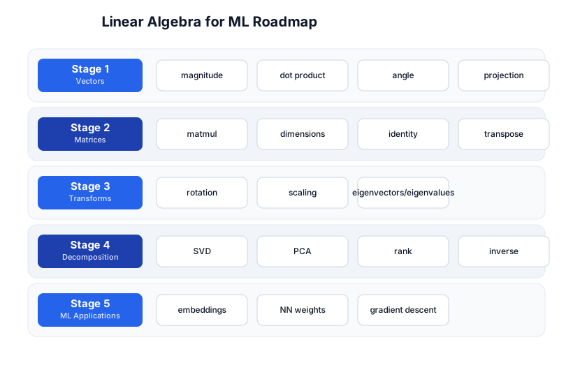
The roadmap moves from vectors (Stage 1), through matrices (Stage 2), transformations (Stage 3), decomposition (Stage 4), and the ML applications that tie it all together (Stage 5).

---

Stage 1 — Vectors

What a vector is

A vector is an ordered list of numbers — a point in space, a direction, or a data point. In ML, a vector is how you represent a data sample (its features) or a learned parameter (a weight vector).

import numpy as np

v = np.array([3, 4])          # a 2D vector
w = np.array([1, 2, 3])      # a 3D vector

Magnitude (length)

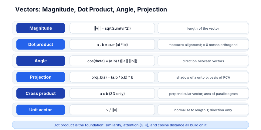
The magnitude (or norm) of a vector is its length: ||v|| = sqrt(sum(vi^2)).

np.linalg.norm(v)             # 5.0 (3-4-5 triangle)

Dot product — the most important operation

The dot product of two vectors measures their alignment: a · b = sum(ai * bi). It’s the foundation of similarity, attention, and projection.

a = np.array([1, 2, 3])
b = np.array([4, 5, 6])
np.dot(a, b)                   # 1*4 + 2*5 + 3*6 = 32

Geometric meaning: a · b = ||a|| ||b|| cos(θ). If the dot product is:

• Positive → vectors point roughly the same direction (acute angle).
• Zero → vectors are orthogonal (perpendicular; 90°).
• Negative → vectors point roughly opposite (obtuse angle).

This is why cosine similarity (dot product of normalized vectors) measures how similar two embeddings are — it’s the cosine of the angle between them.

Angle and cosine similarity

cos_sim = np.dot(a, b) / (np.linalg.norm(a) * np.linalg.norm(b))
# = cos(angle between a and b)
# 1 = identical, 0 = orthogonal, -1 = opposite

Projection

The projection of a onto b is the shadow of a cast onto the line of b:

proj = (np.dot(a, b) / np.dot(b, b)) * b

Projection is how PCA finds the directions of maximum variance — it projects data onto principal axes. It’s also how attention works: the query projects onto the keys.

---

Stage 2 — Matrices

What a matrix is

A matrix is a 2D grid of numbers — a collection of vectors (rows or columns), or a linear transformation (a function that maps vectors to vectors). In ML, a matrix is a weight layer, a batch of data, or a covariance.

A = np.array([[1, 2], [3, 4]])    # 2x2 matrix
B = np.array([[5, 6], [7, 8]])    # 2x2

Matrix multiplication

C = A @ B — the inner dimensions must match: (m × n) @ (n × p) → (m × p). Each element C[i,j] is the dot product of row i of A with column j of B.

C = A @ B                       # (2x2) @ (2x2) -> (2x2)
# [[19, 22],
#  [43, 50]]

Matrix multiplication is composition: applying B then A is A @ B. Order matters — AB ≠ BA in general (non-commutative). This is why the order of layers in a neural network matters.

Key matrix properties

Property	Formula	Meaning
Identity	I: A @ I = A	does nothing (like multiplying by 1)
Transpose	A^T: swap rows/cols	flips the matrix
Inverse	A^-1: A @ A^-1 = I	undoes the transform (if it exists)
Determinant	det(A)	volume scaling factor; 0 = singular (no inverse)

A.T                              # transpose
np.linalg.inv(A)                # inverse (if det != 0)
np.linalg.det(A)                 # determinant
np.eye(3)                        # 3x3 identity

Pitfall: Not every matrix has an inverse. A matrix with det = 0 is singular — its columns are linearly dependent (one is a combination of others). This is why collinear features in ML cause numerical instability.

---

Stage 3 — Linear Transformations

A matrix is a transformation

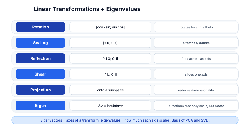
Multiplying a vector by a matrix transforms it: rotates, scales, shears, or projects it. The matrix is the function; the vector is the input.

# rotation by 45 degrees
theta = np.pi / 4
R = np.array([[np.cos(theta), -np.sin(theta)],
              [np.sin(theta),  np.cos(theta)]])
v = np.array([1, 0])
R @ v                            # rotated vector

Transform	Matrix (2D)	Effect
Rotation	[[cos, -sin], [sin, cos]]	rotates by angle θ
Scaling	[[s, 0], [0, s]]	stretches/shrinks
Reflection	[[-1, 0], [0, 1]]	flips
Shear	[[1, k], [0, 1]]	slides one axis
Projection	onto a subspace	reduces dimensionality

Eigenvectors and eigenvalues

An eigenvector of a matrix A is a vector that only scales (doesn’t rotate) when transformed: A v = λ v. The eigenvalue λ is how much it scales.

eigenvalues, eigenvectors = np.linalg.eig(A)
# eigenvalues: the scaling factors
# eigenvectors: the directions that don't rotate

Eigenvectors are the natural axes of a transformation. This is the foundation of PCA (Stage 4) — the principal components are the eigenvectors of the covariance matrix, and the eigenvalues tell you how much variance each captures.

Pitfall: Not every matrix has real eigenvalues. A rotation by 90° has no real eigenvector (every vector rotates). Symmetric matrices (like covariance matrices) always have real eigenvalues — which is why PCA always works.

---

Stage 4 — Decomposition: SVD, PCA, Rank

SVD (Singular Value Decomposition)

SVD decomposes any matrix A into three matrices: A = U Σ V^T:

• U — left singular vectors (output directions)
• Σ — singular values (diagonal; how much each direction matters)
• V^T — right singular vectors (input directions)

U, S, Vt = np.linalg.svd(A)
# A = U @ np.diag(S) @ Vt

SVD is the most general decomposition — it works on any matrix (even non-square, even singular). It reveals the “structure” of the matrix: the singular values tell you the rank (how many independent directions) and the importance of each.

Rank-k approximation

Keep only the top k singular values → a rank-k approximation that captures the most information with the fewest dimensions:

k = 2
A_approx = U[:, :k] @ np.diag(S[:k]) @ Vt[:k, :]
# compresses A to its k most important directions

This is how image compression, denoising, and recommendation systems (Netflix prize) work — truncate to the top-k singular values.

PCA (Principal Component Analysis)

PCA is SVD applied to centered data — it finds the directions (principal components) of maximum variance:

from sklearn.decomposition import PCA
pca = PCA(n_components=2)
X_2d = pca.fit_transform(X)      # 1000D -> 2D, preserving max variance
print(pca.explained_variance_ratio_)  # how much each PC captures

PCA centers the data (subtract the mean), computes the covariance matrix, eigendecomposes it, and projects onto the top-k eigenvectors. It’s SVD on centered data — the same math, applied to find the most informative axes.

Rank

The rank of a matrix is the number of linearly independent rows/columns — the number of genuinely different directions. A rank-1 matrix is an outer product of two vectors; a full-rank square matrix has an inverse. Rank deficiency (rank < dimensions) means redundant information.

Pitfall: PCA assumes linear relationships and that high-variance directions are the most informative. If your data’s structure is non-linear (clusters, manifolds), PCA won’t find it — use t-SNE, UMAP, or an autoencoder instead.

---

Stage 5 — ML Applications

Neural network weights are matrices

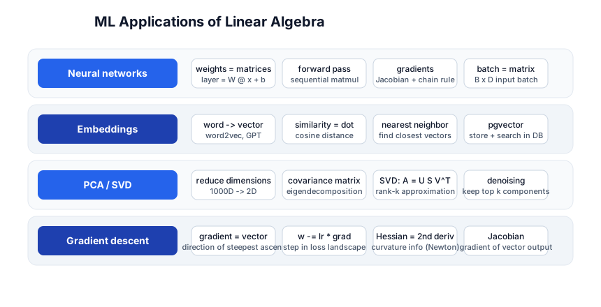
A neural network layer is literally a matrix multiplication + a bias + an activation:

y = activation(W @ x + b)
# W: weight matrix (out_dim x in_dim)
# x: input vector (in_dim)
# b: bias vector (out_dim)
# y: output vector (out_dim)

The forward pass of a deep network is a sequence of matrix multiplications. A batch of B inputs is a B × in_dim matrix, and the layer is W @ X^T (or X @ W^T depending on convention). GPUs are fast at matrix multiplication — this is why deep learning runs on GPUs (and why NVIDIA is worth what it is).

Embeddings are vectors

An embedding (word2vec, GPT, CLIP) turns a discrete object (a word, an image, a user) into a vector in a continuous space where similar things are close. Similarity is the dot product (or cosine), and nearest-neighbor search is finding the closest vectors. The pgvector extension stores and searches these.

Attention is dot products

Self-attention in a transformer is literally batched matrix multiplications of dot products:

Attention(Q, K, V) = softmax(Q @ K^T / sqrt(d)) @ V

Q @ K^T is a matrix of dot products — every query attends to every key. The softmax normalizes to attention weights, then @ V takes the weighted combination. The entire transformer is linear algebra: matrix multiplications, element-wise operations, and nonlinearities.

Gradient descent is vector math

The gradient of the loss is a vector pointing in the direction of steepest ascent. Gradient descent steps in the opposite direction: w -= lr * gradient. The Hessian (second derivative) is a matrix giving curvature information. Stochastic gradient descent, Adam, and all optimizers are linear-algebra operations on the loss landscape.

Covariance and correlation

The covariance matrix of a dataset is X^T X / (n-1) (after centering) — it captures how features vary together. Its eigenvectors are the principal components (PCA). Correlation is normalized covariance. These are the statistics that PCA, factor analysis, and portfolio optimization build on.

---

Quick-Start Checklist

1. Install NumPy — pip install numpy; it’s the linear algebra library for Python.
2. Play with vectors — np.array, np.dot, np.linalg.norm, cosine similarity.
3. Multiply matrices — A @ B; understand the dimension rule and non-commutativity.
4. Compute eigendecomposition — np.linalg.eig on a symmetric matrix; verify A @ v = λ v.
5. Run SVD — np.linalg.svd on a real matrix; reconstruct it from U Σ V^T.
6. Do PCA — sklearn.decomposition.PCA; reduce a high-D dataset to 2D; plot it.
7. Trace a neural network layer — see that nn.Linear is W @ x + b.
8. Understand attention — trace Q @ K^T as a matrix of dot products.
9. Read gradient descent — w -= lr * grad as a vector operation.
10. Use cosine similarity on real embeddings — measure how close two word vectors are.

Common Pitfalls

• Dimension mismatch in matmul — (m × n) @ (n × p); the inner dims must match. The #1 NumPy bug is a shape error from forgetting to transpose.
• Non-commutativity — AB ≠ BA; the order of matrix multiplication matters (and so does the order of neural network layers).
• Singular matrix — det = 0 means no inverse; collinear features cause this and numerical instability.
• Confusing row vs column vectors — NumPy is row-major; v is 1D (no row/column distinction), but v.reshape(-1, 1) makes it a column. Mind the shapes.
• PCA on non-centered data — PCA centers internally, but if you do SVD by hand, center first or the first component is the mean, not a direction of variance.
• Assuming PCA finds non-linear structure — PCA is linear; clusters and manifolds need t-SNE/UMAP/autoencoders.
• Floating point in linear algebra — A @ inv(A) isn’t exactly I due to floating point; use np.allclose not ==.

Further Reading

• 3Blue1Brown: Essence of Linear Algebra — the best visual introduction
• Linear Algebra Done Right by Sheldon Axler — the rigorous textbook
• NumPy Linear Algebra Docs — every function
• Deep Learning Book: Linear Algebra Chapter by Goodfellow et al — LA for DL specifically
• Immersive Math — interactive 3D linear algebra

Related guides

Linear algebra is the math layer under ML and DL — these PyShine tutorials apply it:

• Learn Machine Learning in One Post — PCA, embeddings, and model weights are all linear algebra.
• Learn Deep Learning in One Post — every layer is a matmul; attention is Q·K; gradients are vectors.
• Learn Python in One Post — NumPy is the Python linear algebra library.
• Learn PostgreSQL in One Post — pgvector stores and searches embedding vectors.
• Learn Data Structures and Algorithms in One Post — matrix chain multiplication is a classic DP; graph algorithms use adjacency matrices.

---

Linear algebra is the math that makes ML computable: vectors represent data and parameters, matrices represent transformations, and decompositions reveal structure. The five stages here — vectors, matrices, transformations, decomposition, ML applications — cover everything from a dot product to the attention mechanism in a transformer. The two habits that pay off: always mind the shapes (dimension mismatch is the #1 bug), and think geometrically — a dot product is an angle, a matrix is a transformation, an eigenvector is a natural axis. Open a Python REPL, create two vectors, take their dot product, compute the cosine similarity, and watch a · b / (||a|| ||b||) give you the angle between them — once you see the geometry, the algebra makes sense.

Enjoyed this post? Never miss out on future posts by following us