Needle 2: A 14MB Foundation Model for Tiny Devices

Needle 2 is an open 45-million-parameter model built by Cactus Compute that does one thing exceptionally well: tool calling. The entire model, weights and engine combined, ships as a single 14MB binary that runs a full session in approximately 28MB of RAM. That is smaller than a typical podcast MP3. It trades wins on benchmarks with models 5x to 70x larger – FunctionGemma 270M, LFM2.5 230M, and Apple FM – while using only 2 bits per weight against their 16-bit floating point.

This is not a general-purpose chatbot. Needle 2 is a specialist: it reads your tool descriptions, decides which function to call, fills in the arguments, and returns structured JSON. No free text, no hallucinated answers, no network round-trip. It runs entirely on-device, offline, in milliseconds, for free after installation.

The Problem Needle 2 Solves

Cloud-based tool calling through APIs like OpenAI or Anthropic has three fundamental limitations: latency from network round-trips, metered cost per token, and privacy exposure of user data. For applications running on phones, wearables, smart home hubs, or robots, these limitations are dealbreakers. A thermostat that needs to call a cloud API to interpret “make it cooler” is a thermostat that fails when the internet goes down.

Needle 2 addresses this by compressing the entire inference pipeline – model weights, tokenizer, and C++ execution engine – into a single self-contained binary that can be deployed across 16 platform targets including Android, iOS, macOS, Windows, Linux, WebAssembly, watchOS, and even RISC-V and MIPS architectures.

Simple Attention Network Architecture

Needle 2 is built on the Simple Attention Network recipe, a dense small-model architecture documented in the paper “A Controlled Study of Attention-Only Transformers” (arXiv:2607.18363). The core finding: feed-forward networks hold two thirds of a transformer’s non-embedding parameters, yet when the freed budget is reallocated into attention depth, the quality gap shrinks to 0.006 nats – about a quarter of one percent of loss.

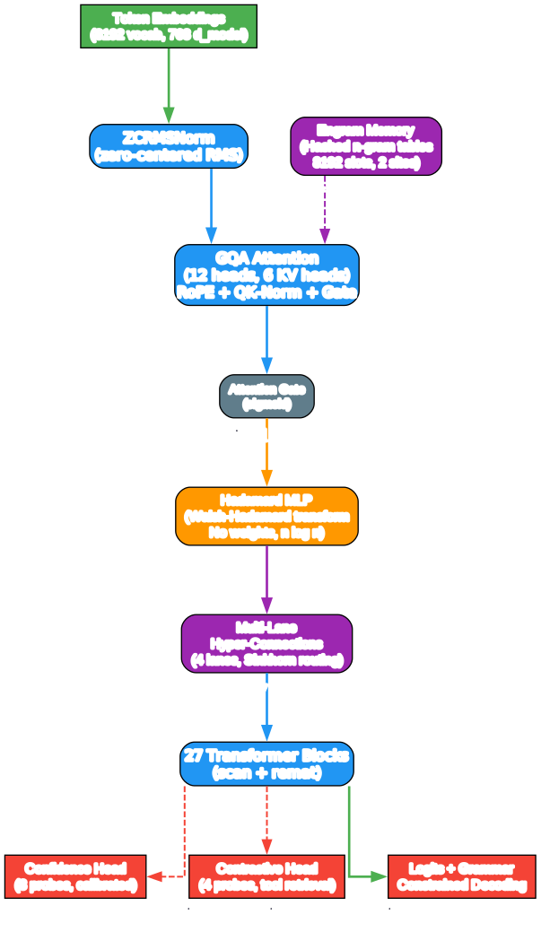
Understanding the Architecture

The architecture diagram above illustrates the core components of Needle 2’s Simple Attention Network. Let us break down each component:

Token Embeddings and Vocabulary The model uses an 8192-token vocabulary with a 768-dimensional embedding space. This is deliberately small – a typical LLM vocabulary might use 50,000+ tokens, but Needle 2 serves tool calling, not general text generation, so the vocabulary can be compact without sacrificing task quality.

ZCRMSNorm (Zero-Centered RMS Normalization) Every layer begins with a zero-centered RMS normalization step. Unlike standard LayerNorm which subtracts the mean, ZCRMSNorm operates on the RMS (root mean square) of the input, applying a learned scale parameter initialized to zero. This keeps the normalization numerically stable during early training and is cheaper to compute than full LayerNorm.

GQA Attention (Grouped Query Attention) The attention mechanism uses 12 query heads but only 6 key-value heads, following the GQA pattern. Each head applies Rotary Position Embedding (RoPE) with theta=100000, followed by QK-normalization – the technique the paper credits with keeping 48-layer attention-only stacks trainable. A sigmoid gate on the attention output allows the model to dynamically suppress attention when the Hadamard MLP path is more informative.

Engram Memory (Hashed n-gram Key-Value Tables) This is one of the most novel components. Instead of relying solely on the KV cache for memory, Needle 2 embeds hashed n-gram lookup tables at two specific layers (layers 2 and 15). These “engram” tables use 8192 slots and gather key-value rows based on FNV-style hash indices computed from token n-grams. The engram sites fire with a learned attention-like gate that determines how much external memory to inject at each position. This gives the model a form of associative recall that does not grow with sequence length.

Hadamard MLP (Walsh-Hadamard Transform) The traditional FFN is replaced entirely. Instead of two large weight matrices, the Hadamard MLP applies the orthonormal Walsh-Hadamard transform – a fixed mathematical matrix with no learnable parameters – in O(n log n) time. Three learned diagonal vectors (d1, d2, d3) gate the signal before and after each transform. This eliminates roughly two thirds of the model’s parameters while preserving the mixing capacity the FFN would provide.

Multi-Lane Hyper-Connections (mHC) Instead of a single residual stream, Needle 2 maintains 4 parallel “lanes” per layer. The mHC system learns input-dependent routing between these lanes using a Sinkhorn-normalized doubly-stochastic matrix, ensuring balanced allocation of information across lanes. Each lane gets its own pre-attention gate, post-attention gate, and residual mixing matrix, all parameterized compactly.

Confidence and Contrastive Heads Two auxiliary heads sit on top of the stack. The Confidence Head uses 8 learned probes to pool hidden states and produce a calibrated confidence score for each generated call. The Contrastive Head uses 4 probes to embed both queries and tool descriptions into a shared 128-dimensional space, enabling tool retrieval at inference time.

27 Transformer Blocks with Scan and Remat All 27 layers share parameters via JAX’s scan primitive with gradient rematerialization, keeping memory usage flat regardless of depth. The layer stack processes 4 lanes in parallel, averaging them at the final norm to produce the output logits.

Grammar-Constrained Decoding The final output is constrained by a byte-level grammar compiled from the declared tool schemas. This means the model can only emit tokens that produce valid JSON matching your tool definitions. The JSON cannot be malformed by construction.

Cactus Quants (CQ) Compression Pipeline

The journey from a 90MB FP16 checkpoint to a 14MB binary is the work of Cactus Quants, a custom quantization system that achieves 6.4x compression with minimal quality loss.

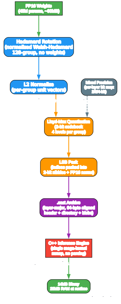
Understanding the Quantization Pipeline

The diagram above traces the compression pipeline from FP16 weights to the final deployable binary. Here is how each stage works:

FP16 to Hadamard Rotation The process begins with the full-precision FP16 weights totaling approximately 90MB for 45M parameters. The first transformation applies a normalized Walsh-Hadamard matrix to each group of 128 weights. This rotation is critical: it spreads the energy of each weight across all dimensions equally, making the distribution more uniform and thus more amenable to quantization. The Hadamard matrix is orthonormal and fixed (no learned parameters), computed in O(n log n) time.

L2 Normalization After rotation, each 128-element group is normalized to unit length. The L2 norm of each group is stored separately as an FP16 scalar. This separates the “direction” of each weight group (which gets quantized) from its “magnitude” (which stays in full precision). The insight: direction is low-entropy and compresses well, while magnitude carries the critical scaling information.

Lloyd-Max Quantization on the Unit Sphere The unit-normalized vectors are quantized using Lloyd-Max scalar quantization, an optimal quantizer for a known distribution. Since the Hadamard-rotated, normalized vectors follow a distribution close to a Gaussian on the unit sphere, the Lloyd-Max codebook is precomputed offline for Gaussian distributions at 2, 3, and 4 bits. A 2-bit codebook has 4 levels, a 3-bit has 8, and a 4-bit has 16. The codebook is shared across all weights in the model, stored once in the binary header.

LSB Packing The quantized indices are packed into a contiguous bitstream using LSB-first packing. For 2-bit quantization, every 8 consecutive indices are packed into a 2-byte word. For ternary quantization (1.58 bits, 3 levels), 2-bit “crumbs” are packed four per byte with codes 3, 0, 1 representing trit indices 0, 1, 2. This packing is what the C++ inference engine reads directly via mmap – no parsing, no decoding step.

The .cact Archive Format The packed indices, per-group norms, and all non-quantized tensors (norms, gates, Hadamard diagonals) are assembled into the .cact binary format. The layout is layer-major: the embedding, then all tensors for layer 0, then layer 1, and so on. This ensures the working set for any single layer is contiguous in memory, maximizing cache locality. A 120-byte header carries the full architecture geometry, followed by a nameless tensor directory, then 64-byte aligned tensor blobs. The engine reads the geometry from the header and indexes tensors by position, so one binary format loads and runs any configuration of the architecture.

Mixed Precision The format supports per-layer mixed precision through a bits map: some layers can be 2-bit, others 3 or 4-bit, based on sensitivity analysis. The bits map is stored in the checkpoint and rides in the binary, so the engine always knows exactly how to decode each tensor.

The C++ Inference Engine The final binary is not just weights – it includes a compiled C++ inference engine, a single mega-kernel that reads the .cact format directly via memory-mapped I/O. There is no model loading step, no parsing, no framework initialization. The binary is the model. On first run, the Python package fetches the platform-specific engine from Hugging Face and caches it. All subsequent inference is completely offline.

Tool Calling: The Agentic Loop

Needle 2 approaches every problem as a function call. The context declares what may be called; the model answers with calls. There is no free-text fallback – if no declared tool can serve a request, the model returns the empty call [], which is the entire contract for off-topic input.

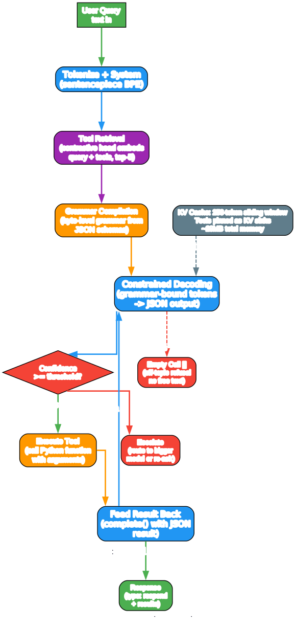
Understanding the Tool Calling Loop

The diagram above shows the complete agentic loop from user query to final response. Here is a detailed walkthrough:

Tokenization and System Context The user’s query text is tokenized using a custom SentencePiece BPE tokenizer with an 8192-token vocabulary. An optional system turn carries environment facts (date, locale, device, battery level, network status, location) as structured key-value pairs, not instructions. The model resolves relative language against these facts: “tomorrow at 7” becomes an absolute time only when a date: fact is present.

Tool Retrieval via Contrastive Head When the declared tool catalogue has more than five tools, the contrastive head engages automatically. At initialization, every tool schema is embedded once by the built-in contrastive head into a 128-dimensional space. Each turn embeds the query the same way, and only the five highest-scoring tools enter the context. The grammar is then rebuilt over just that subset, so an unselected tool is unreachable, not merely unlikely. For five or fewer tools, retrieval is bypassed and all tools are included directly.

Grammar-Constrained Decoding This is where Needle 2 diverges fundamentally from LLM-based tool callers. Before generation begins, the declared tool schemas are compiled into a byte-level grammar. This grammar constrains every token the model can emit: the output must be valid JSON, with the correct tool name, correct argument names, and argument values that satisfy any declared constraints (ranges, patterns, enumerations, length limits). The model cannot produce malformed JSON by construction – the grammar makes it impossible.

Confidence Gating Every response carries a calibrated confidence score, computed as the minimum of two signals: a learned confidence head that scores the full prompt plus the generated call, and the decoding probability of the call tokens. A call is accepted only when both signals agree. The contract is simple: set a threshold for your application, act at or above it, escalate or re-ask below it. The failure mode is escalation, not wrong execution.

Execution and Feedback When a call is accepted, Needle executes the corresponding Python function with the parsed arguments. The result is serialized as JSON and fed back into the next complete() call. The model continues from this result, and later arguments may depend on earlier results – for example, search_for_contact first, then send_instant_message with the returned contact_id. A final "type": "respond" with empty function calls signals the loop is done.

Bounded Memory: 256-Token Sliding Window The KV cache uses a 256-token sliding window, with the declared tool schemas pinned as KV sinks. This means the tools are always in context, but the conversation history slides. Total memory stays near 28MB regardless of how long the conversation runs. The window width is computed from a fixed KV budget of approximately 11MB, ensuring the memory footprint is predictable and bounded.

Off-Topic Refusal If no declared tool can serve the request, the model returns the empty call []. This is not an error – it is the designed response for off-topic input. There is no free-text generation, no “I’m sorry, I can’t help with that” – just a structured empty call that your application logic can handle programmatically.

Installation and Quickstart

pip install cactus-needle

The package is available on PyPI as cactus-needle. The inference engine is fetched once from Hugging Face on first use and cached locally. All subsequent inference runs entirely offline.

Simple Tool Calling

import needle

@needle.tool
def get_weather(city: str):
    "Get the current weather for a city."
    return {"city": city, "temp_c": 27, "sky": "clear"}

agent = needle.Needle(tools=[get_weather])
print(agent.run("what's it like in Lagos right now?")["results"])
# [{'city': 'Lagos', 'temp_c': 27, 'sky': 'clear'}]

The @needle.tool decorator reads the function signature for argument types and the docstring for descriptions. The run() method completes the full agentic loop: the model picks the call, Needle executes your function, feeds the result back, and returns the final response with executed tool results attached.

Structured Extraction

from pydantic import BaseModel

class Invoice(BaseModel):
    vendor: str
    total: float
    due_date: str

invoice = needle.extract("Invoice from Acme Corp, $1,200.00, due 2026-09-01", Invoice)
print(invoice.vendor, invoice.total)   # -> Acme Corp 1200.0

Extraction is not a separate mode – it is tool calling with one tool. Declare the record as the only schema and pass the content where the query goes. With one declared tool, the grammar admits exactly one call of that name, so schema conformance is guaranteed rather than requested.

Constrained Arguments

from typing import Annotated, Literal

@needle.tool
def send_money(
    amount: Annotated[float, needle.Field(gt=0, le=10000, description="USD, up to 10,000")],
    to:     Annotated[str,   needle.Field(pattern=r"^@[a-z0-9_]+$", description="recipient handle")],
    memo:   Annotated[str,   needle.Field(max_length=80)] = "",
):
    "Send money to a handle."
    return {"sent": amount, "to": to}

The Field constraints – ranges, patterns, enumerations, length limits – are compiled directly into the decode grammar. The model can only emit values that satisfy them. A Literal type becomes a fixed set the model must choose from; it cannot emit anything else.

Fine-Tuning with LoRA

Needle 2 fine-tunes with LoRA adapters on the frozen base model: rank 16 on the five attention projections of every layer, trained on your JSONL data, then merged into the weights at export. The engine, tokenizer, and confidence head are untouched.

Data Format

{"query": "dim the kitchen to 10", "tools": [{"name": "set_lights", "parameters": {"type": "object", "properties": {"room": {"type": "string"}, "brightness": {"type": "integer"}}, "required": ["room"]}}], "answers": [{"name": "set_lights", "arguments": {"room": "kitchen", "brightness": 10}}], "reasoning": "'kitchen' -> room; 'dim to 10' -> brightness 10"}

Each line is one example: query and tools describe the turn, answers lists the exact calls the model should emit, and reasoning is a short derivation of each argument from its source span. Include off-topic examples with "answers": [] – without them, the tuned model will try to call a tool on everything.

Training Commands

# LoRA fine-tune on your data
needle finetune data.jsonl --epochs 10

# Generate synthetic data via OpenRouter (optional)
needle generate-data --tools my_tools.json --num-samples 500 --output data.jsonl

# Build a tuned .cact binary (merges adapter into base)
needle build checkpoints/needle2.pkl --lora checkpoints/needle_lora.pkl --out my_needle.cact

# Run the tuned model
python -c "import needle; agent = needle.Needle(weights='my_needle.cact', tools=[...]); print(agent.run('...'))"

Training is plain JAX and runs on any accelerator JAX supports. On NVIDIA machines, install the CUDA build: pip install "cactus-needle[gpu]". On Apple Silicon, use the metal extra: pip install "cactus-needle[metal]". Training runs in float32 on every backend.

Key Fine-Tuning Insights

• Tool selection moves first: a few hundred clean examples measurably improve which tool gets picked
• Argument grounding needs more data: on the order of thousands of examples with reasoning lines and varied phrasings
• Step count matters: 200 examples at batch 16 is only 13 steps per epoch; the default 3 epochs is 39 steps total, which barely moves a rank-16 adapter. For small datasets, run 10 to 30 epochs
• The confidence head is not updated: fine-tuning does not update the calibration head, so tuned weights report confidence as None

Deployment: 16 Platform Targets

The 14MB binary runs across an extraordinary range of hardware, from high-end desktops to embedded microcontrollers.

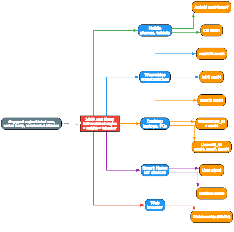
Understanding the Deployment Landscape

The diagram above maps the deployment ecosystem for Needle 2. The single 14MB .cact binary serves as the universal deployment artifact across all platforms:

Mobile (Android and iOS) Android targets both arm64 and armv7 architectures, covering the vast majority of Android devices in circulation. iOS targets arm64, the architecture used by every iPhone and iPad since the iPhone 5S. The binary loads via the platform’s native shared library mechanism, with no JIT compilation or framework initialization overhead.

Wearables (watchOS and tvOS) Apple Watch (watchOS arm64) and Apple TV (tvOS arm64) are first-class targets. A 14MB binary with 28MB RAM usage is well within the memory budget of modern smartwatches, which typically have 1GB or more of RAM. This enables on-watch tool calling for home automation, health tracking, and voice commands without phone tethering.

Desktop (macOS, Windows, Linux) All three major desktop platforms are supported across multiple architectures: macOS on arm64 (Apple Silicon), Windows on both x86_64 and arm64, and Linux on x86_64, arm64, armv7, riscv64, and mipsel. The Linux builds include both glibc (manylinux) and musl variants, covering Alpine Linux containers and embedded distributions.

Smart Home and IoT The mipsel and musllinux targets open the door to MIPS-based IoT devices and Alpine Linux-based embedded systems. The musl target is particularly important for Docker containers, which frequently use Alpine Linux for its small base image size.

WebAssembly (WASM) The WASM target allows Needle 2 to run entirely in a browser tab. The 14MB binary downloads once and is cached by the browser. All inference happens client-side – no server, no API key, no data leaving the user’s device. This is particularly valuable for privacy-sensitive applications like form filling, data extraction, and command parsing.

Air-Gapped Deployment For devices that must never touch the network, the engine is fetched once on a connected machine and transferred to the device. Three methods: needle fetch downloads the engine for the current platform; copy the file to the same cache path on the device; or set NEEDLE_LIB_PATH to point directly at the file. With HF_HUB_OFFLINE=1, the package fails fast with a clear error if the engine is missing, rather than attempting a network download.

The Response Contract

Every complete() call returns one JSON object:

{
  "type": "call",
  "success": true,
  "error": null,
  "function_calls": [
    {
      "name": "set_lights",
      "arguments": {"room": "living room", "on": true, "brightness": 30}
    }
  ],
  "reasoning": "'living room' -> room; 'dim' -> on true, brightness 30",
  "confidence": 0.94,
  "prefill_tps": 4300.0,
  "decode_tps": 850.0,
  "peak_ram_mb": 28.5
}

The type field is either "call" (the model wants to execute tools) or "respond" (the loop is done). The reasoning field shows the model’s derivation of each argument from its source span in the query. The confidence field carries the calibrated score. Performance metrics (prefill_tps, decode_tps, peak_ram_mb) are reported on every response, so you can monitor inference quality in production.

Key Features Summary

Feature	Description
Self-contained	Weights baked into a single 14MB engine binary; no separate model files
Grammar-constrained	Byte-level grammar from JSON schemas constrains every decoded token
Confidence-gated	Calibrated confidence head; set threshold, act above, escalate below
Tool retrieval	Contrastive head selects top-5 tools per turn from large catalogues
Bounded memory	256-token sliding window with tools pinned as KV sinks; ~28MB total
LoRA fine-tuning	Rank-16 adapters on frozen base; merged at export to single .cact
Mixed precision	Per-layer bit map: 2/3/4-bit CQ quantization
16 platform targets	Android, iOS, macOS, Windows, Linux, WASM, watchOS, tvOS, RISC-V, MIPS

Troubleshooting

Issue	Cause	Solution
FileNotFoundError on first run	Engine not cached	Run needle fetch or ensure network access on first run
failed to load weights	.cact format version mismatch	Rebuild with current package version: needle build
Loss goes NaN on CPU	Fixed in newer versions	pip install --upgrade cactus-needle
Tuned model answers everything with empty call	Undertrained or too few examples	Run 10-30 epochs; add off-topic examples with answers: []
Correct tool but wrong arguments	Dataset too small or uniform	Add thousands of examples with reasoning lines and varied phrasings
Low confidence on correct calls	Confidence head calibrated for base model only	Tuned weights report confidence: null; use base model for calibration

Conclusion

Needle 2 represents a fundamentally different approach to on-device AI: instead of shrinking a large model, it was designed from the ground up for tiny devices. The Simple Attention Network architecture eliminates the FFN entirely, the Hadamard MLP replaces it with a weightless mathematical transform, Cactus Quants compresses weights to 2 bits on the unit sphere, and grammar-constrained decoding guarantees structured output by construction.

The result is a 14MB binary that runs in 28MB of RAM, deploys to 16 platform targets including watches and browsers, and trades wins with models 5x to 70x larger on tool-calling benchmarks. For any application that needs structured decisions on a device too small, too private, or too offline for a cloud API, Needle 2 is a compelling option.

Links

• GitHub: github.com/cactus-compute/needle
• PyPI: pypi.org/project/cactus-needle
• HuggingFace Weights: huggingface.co/Cactus-Compute/needle2
• Paper: arxiv.org/abs/2607.18363

Related Posts

• Cognee: Open Source AI Memory Platform for Agents
• TencentDB Agent Memory: Local Long-Term Memory for AI Agents
• ZeroStack: Minimal Rust Coding Agent for Memory Performance

Enjoyed this post? Never miss out on future posts by following us