Stable-WorldModel: Reproducible World Model Research with Model-Predictive Control

World model research with model-predictive control has long suffered from fragmentation – researchers must build their own data pipelines, environment wrappers, planning solvers, and evaluation protocols, making it nearly impossible to compare results across papers. Stable-WorldModel, from a team including Yann LeCun, is an open-source Python platform that solves this problem by providing a unified interface for the three stages of world model research – collecting data, training, and evaluating with model-predictive control – across 30+ standardized environments with controllable factors of variation, 7 planning solvers, and 5 data formats.

How It Works

Stable-WorldModel organizes the entire world model research lifecycle into a three-stage pipeline: Collect, Train, and Evaluate. Each stage is accessible through a single World class that handles environment stepping, policy invocation, data recording, and success tracking.

Stable-WorldModel Architecture

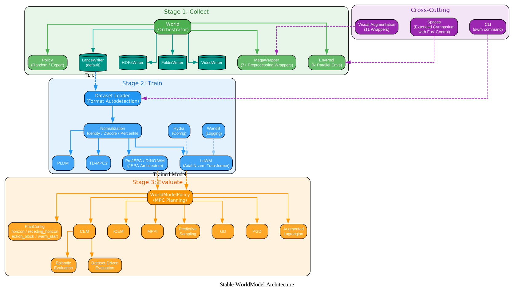
The architecture diagram above shows the three-stage pipeline and how components connect. In Stage 1 (Collect), the World class orchestrates data collection through EnvPool (managing N parallel environments) and MegaWrapper (applying 7+ preprocessing wrappers). A Policy drives the rollout loop, and data is written to one of 5 format backends. LanceDB is the default, delivering 3.4x faster throughput than HDF5 (4,815 vs 1,416 samples/s) and 3.2x smaller storage (13.3 GB vs 43.1 GB). In Stage 2 (Train), datasets are loaded via the format registry with autodetection. Normalization scalers (Identity, ZScore, Percentile) preprocess data. World model implementations include LeWM (encoder-predictor with AdaLN-zero conditioning), PreJEPA/DINO-WM (JEPA architecture with video encoding), PLDM, TD-MPC2, and behavior cloning baselines (GCBC, GCIVL, GCIQL). Training uses Hydra for configuration and WandB for logging. In Stage 3 (Evaluate), WorldModelPolicy implements MPC planning with action buffering and warm-starting. It delegates to a Solver (CEM, iCEM, MPPI, etc.) that optimizes action sequences using the world model’s get_cost() method. Two evaluation modes are available: episodic (random goals, auto-reset) and dataset-driven (start/goal from trajectories, guaranteed solvable). The Cross-cutting Components include Spaces (extended Gymnasium spaces with state tracking and FoV control), the CLI (swm command for dataset inspection, environment listing, and format conversion), and Visual Augmentation wrappers (11 types with schedule functions for domain randomization).

The World._run_iter() method drives the rollout loop, calling envs.step() in parallel across all environments. The MegaWrapper chains 7+ wrappers – EnsureInfoKeysWrapper, EnsureImageShape, EnsureGoalInfoWrapper, EverythingToInfoWrapper, MapKeysWrapper, AddPixelsWrapper, and ResizeGoalWrapper – into a single preprocessing pipeline. The PlanConfig dataclass controls MPC behavior with parameters like horizon (planning horizon), receding_horizon (steps to execute before replanning), action_block (action repeat/frame skip), and warm_start (reuse previous plan as initialization).

This architecture serves as a “research infrastructure layer” that lets researchers focus on model design rather than reinventing data pipelines, environment wrappers, and evaluation protocols for every experiment.

Key Insight: Stable-WorldModel’s World class is the single orchestrator that bundles EnvPool (vectorized parallel environments), MegaWrapper (7+ preprocessing wrappers), and a rollout loop into one interface. The collect() method records episodes to LanceDB/HDF5/Video, while evaluate() runs policies with automatic reset handling and success tracking – meaning researchers never need to write environment stepping loops again.

Key Features

Stable-WorldModel provides a comprehensive feature set designed for reproducible world model research:

Feature	Description
Unified 3-Stage Pipeline	Collect data, train models, and evaluate with MPC – all through a single `World` interface
30+ Environments	DeepMind Control Suite, Gymnasium, OGBench, Craftax, ALE, PushT, TwoRoom with controllable factors of variation
Factors of Variation	Independently control visual and physical parameters (colors, shapes, sizes, dynamics, morphology) for zero-shot generalization testing
7 Planning Solvers	CEM, iCEM, MPPI, Predictive Sampling, GD, PGD, Augmented Lagrangian – all implementing the `Solver` protocol
5 Data Formats	LanceDB (default, 3.4x faster than HDF5), HDF5, Folder, Video, LeRobot – with one-shot conversion
World Model Baselines	LeWM (AdaLN-zero Transformer), PreJEPA/DINO-WM (JEPA), PLDM, TD-MPC2, GCBC, GCIVL, GCIQL
Visual Augmentation	11 wrappers: ChromaKey, Noise, ColorJitter, Blur, Occlusion, MovingPatch, RandomShift, Cutout, RandomConv, Grayscale, Resolution
CLI	`swm` command for datasets, environments, checkpoints, and format conversion
LeRobot Integration	Read-only adapter for LeRobot Hub datasets (Python 3.12+)

Stable-WorldModel Features

The features diagram shows how Stable-WorldModel’s capabilities radiate from a central hub. The Unified Pipeline provides collect(), evaluate(), and reset() methods that handle environment stepping, policy invocation, data recording, and success tracking. The 30+ Environments span from DeepMind Control Suite (Cheetah, Hopper, Walker, etc.) to Gymnasium classic control, OGBench manipulation, Craftax, ALE Atari, and custom benchmarks (PushT, TwoRoom). All follow the Gymnasium API. Factors of Variation expose a variation_space describing controllable parameters. A single world.reset(options={'variation': ['all']}) randomizes everything, and exact values can be set for reproducibility. The 7 Solvers all implement the Solver protocol with configure() and __call__(). 5 Data Formats include LanceDB (default, append-friendly, fast indexed reads), HDF5 (portable single-file), Folder (inspection-friendly), Video (compact MP4 episodes), and LeRobot (read-only Hub adapter). One-shot conversion is available via swm.data.convert(). World Model Baselines include LeWM (encoder-predictor with AdaLN-zero conditioning in Transformer blocks), PreJEPA/DINO-WM (JEPA architecture with video encoding and action-conditioned rollout), PLDM, TD-MPC2, GCBC, GCIVL, and GCIQL. Visual Augmentation offers 11 wrappers with schedule functions (constant, linear, cosine, exponential, sinusoidal) for curriculum learning. The CLI provides swm datasets, swm inspect, swm envs, swm fovs, swm checkpoints, and swm convert for zero-code dataset and environment management. LeRobot Integration enables training on existing robotics datasets with a single swm.data.load_dataset("lerobot://lerobot/pusht") call.

These features work together as a cohesive research platform, enabling reproducible benchmarks, domain randomization experiments, and zero-shot generalization evaluation without custom infrastructure.

Amazing: The platform ships with 30+ environments each equipped with independently controllable factors of variation – colors, shapes, sizes, dynamics, and morphology – enabling zero-shot generalization testing without any additional setup. A single world.reset(seed=0, options={'variation': ['all']}) call randomizes every visual and physical parameter, and you can set exact values like variation_values={'agent.color': np.array([255, 0, 0])} for precise domain randomization experiments.

Installation

Install Stable-WorldModel with pip:

      
        # Base install (core only)
pip install stable-worldmodel

# Full install (training, environments, data formats)
pip install 'stable-worldmodel[all]'

# LeRobot support (requires Python 3.12+)
pip install 'stable-worldmodel[lerobot]'

Or install from source:

      
        git clone https://github.com/galilai-group/stable-worldmodel.git
cd stable-worldmodel
uv venv --python=3.10
uv sync --extra all --group dev

The default data directory is ~/.stable_worldmodel/, configurable via the $STABLEWM_HOME environment variable.

Usage

Quick Start

      
    
      
        import stable_worldmodel as swm
from stable_worldmodel.policy import WorldModelPolicy, PlanConfig
from stable_worldmodel.solver import CEMSolver

# 1. Collect a dataset
world = swm.World("swm/PushT-v1", num_envs=8)
world.set_policy(your_expert_policy)
world.collect("data/pusht_demo.lance", episodes=100, seed=0)

# 2. Load and train
dataset = swm.data.load_dataset("data/pusht_demo.lance", num_steps=16)

# 3. Evaluate with MPC
solver = CEMSolver(model=world_model, num_samples=300)
policy = WorldModelPolicy(solver=solver, config=PlanConfig(horizon=10))
world.set_policy(policy)
results = world.evaluate(episodes=50)
print(f"Success Rate: {results['success_rate']:.1f}%")

      
      
        

Data Collection

      
        import stable_worldmodel as swm

world = swm.World("swm/PushT-v1", num_envs=8, image_shape=(224, 224))

# Attach a random policy for data collection
policy = swm.policy.RandomPolicy(seed=42)
world.set_policy(policy)

# Collect 100 episodes to LanceDB (default, recommended)
world.collect("data/pusht_random.lance", episodes=100, seed=0)

# Re-running extends the dataset (mode='append' is default)
world.collect("data/pusht_random.lance", episodes=50, seed=1)  # +50 episodes

# Or collect to video format (compact, one MP4 per episode)
world.collect("data/pusht_random_video", episodes=100, seed=0,
              format="video")

Loading Data and Format Conversion

      
    
      
        import stable_worldmodel as swm

# Load dataset (format autodetected from path)
dataset = swm.data.load_dataset(
    "data/pusht_random.lance",
    num_steps=16,
    keys_to_load=["pixels", "action", "state"],
)

sample = dataset[0]
print(sample["pixels"].shape)   # (16, 3, H, W)
print(sample["action"].shape)   # (16, action_dim)

# Convert between formats
swm.data.convert(
    "data/pusht_random.lance",       # source
    "data/pusht_random_video",       # destination
    dest_format="video",
    fps=30,
)

# Load from LeRobot Hub (requires Python 3.12+)
# dataset = swm.data.load_dataset(
#     "lerobot://lerobot/pusht",
#     primary_camera_key="observation.images.top",
#     num_steps=4,
# )

      
      
        

Factors of Variation

      
    
      
        import stable_worldmodel as swm
import numpy as np

world = swm.World("swm/PushT-v1", num_envs=4, image_shape=(224, 224))

# View the variation space structure
print(world.envs.single_variation_space.to_str())
# Output shows: agent.color, agent.scale, agent.shape, block.color, etc.

# Randomize specific factors at reset
world.reset(seed=0, options={"variation": ["agent.color", "block.color"]})

# Randomize everything
world.reset(seed=0, options={"variation": ["all"]})

# Set exact values for domain randomization experiments
world.reset(seed=0, options={
    "variation": ["agent.color", "background.color"],
    "variation_values": {
        "agent.color": np.array([255, 0, 0], dtype=np.uint8),      # Red agent
        "background.color": np.array([0, 0, 0], dtype=np.uint8),    # Black bg
    }
})

      
      
        

Stable-WorldModel MPC Pipeline

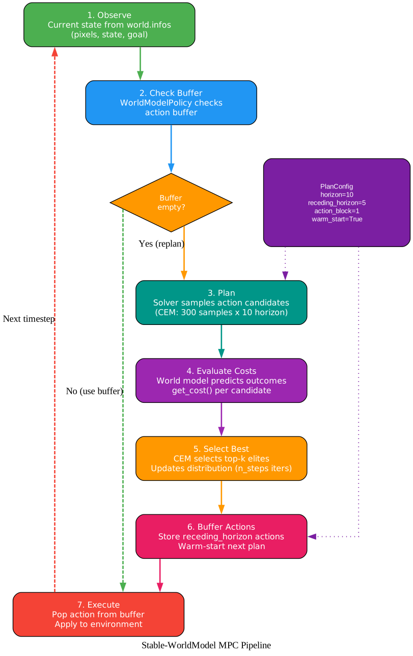
The MPC pipeline diagram illustrates the 7-step model-predictive control loop. Step 1 (Observe): The environment produces an observation stored in world.infos, a dictionary containing pixels, state, goal, and other keys. The MegaWrapper ensures all keys are present and properly formatted. Step 2 (Check Buffer): WorldModelPolicy checks its action buffer. If the buffer has actions remaining from a previous plan, it pops the next action and skips replanning. If the buffer is empty (or after an episode reset via _needs_flush), it triggers the replanning process. Step 3 (Plan): The solver (e.g., CEM) samples action candidates. For CEM with 300 samples and horizon 10, this creates a tensor of shape (n_envs, 300, 10, action_dim). If warm_start=True, the remaining actions from the previous plan initialize the distribution mean. Step 4 (Evaluate Costs): The world model’s get_cost() method predicts outcomes for each action candidate. It receives the current observation and all candidate action sequences, returning a cost tensor of shape (n_envs, num_samples). Lower cost means better predicted outcome. Step 5 (Select Best): CEM selects the top-k (e.g., 30) lowest-cost candidates as “elites.” The distribution mean and variance are updated to these elites. This process repeats for n_steps iterations (e.g., 30), progressively refining the action distribution. Step 6 (Buffer Actions): The final plan (first receding_horizon actions) is stored in the action buffer. If warm_start=True, the remaining actions beyond the receding horizon are saved as initialization for the next plan. This avoids cold-starting the solver from scratch each time. Step 7 (Execute): The first action is popped from the buffer and applied to the environment via envs.step(). The environment returns new observations, rewards, and termination flags. The loop continues from Step 1.

The decision diamond “Buffer empty?” after Step 2 determines whether to replan or execute a buffered action. This is the core of receding horizon control – plans are computed for a horizon but only executed for a few steps before replanning. Compared to model-free approaches, MPC with warm-starting is more sample-efficient because it reuses information from previous plans. The PlanConfig parameters (shown in the side panel) control this behavior: horizon=10 sets the planning horizon, receding_horizon=5 determines how many steps to execute before replanning, action_block=1 sets the action repeat, and warm_start=True enables plan reuse.

Takeaway: With just pip install stable-worldmodel, you get a complete world model research pipeline: 30+ environments with factors of variation, 7 planning solvers (CEM, iCEM, MPPI, GD, PGD, Augmented Lagrangian), 5 data formats with LanceDB delivering 3.4x faster throughput than HDF5, reference implementations of LeWM and DINO-WM, and a CLI for dataset inspection and format conversion – all accessible through a single World interface.

Solvers and Planning

The Solver protocol defines the planning interface with two key abstractions: Costable (cost function interface with criterion() and get_cost()) and Solver (planning interface with configure() and __call__()). This clean separation allows researchers to swap solvers without modifying the world model or evaluation pipeline.

The CEM (Cross-Entropy Method) solver is the most commonly used. It works by sampling num_samples action candidates from a parameterized distribution, evaluating costs via the world model, selecting the top-k lowest-cost candidates as “elites,” and updating the distribution to these elites. This process repeats for n_steps iterations, progressively refining the action distribution toward optimal trajectories.

      
    
      
        import stable_worldmodel as swm
from stable_worldmodel.policy import WorldModelPolicy, PlanConfig
from stable_worldmodel.solver import CEMSolver

# Load your trained world model
world_model = swm.policy.AutoCostModel("checkpoints/lewm-pusht")

# Create a CEM solver
solver = CEMSolver(
    model=world_model,
    num_samples=300,
    n_steps=30,
    topk=30,
    device="cuda",
)

# Configure MPC planning
config = PlanConfig(
    horizon=10,             # Planning horizon
    receding_horizon=5,     # Steps to execute before replanning
    action_block=1,         # Action repeat / frame skip
    warm_start=True,        # Reuse previous plan as initialization
)

# Create planning policy
policy = WorldModelPolicy(solver=solver, config=config)

# Evaluate
world = swm.World("swm/PushT-v1", num_envs=1, image_shape=(224, 224))
world.set_policy(policy)
results = world.evaluate(episodes=50, seed=0)
print(f"Success Rate: {results['success_rate']:.1f}%")

      
      
        

The WorldModelPolicy manages action buffering and receding horizon execution. When warm_start=True, the remaining actions from the previous plan initialize the next planning iteration, significantly improving sample efficiency. The action_block parameter controls how many times each action is repeated before the next planning step, effectively implementing frame skipping.

CLI Usage

      
        # List all cached datasets
swm datasets

# Inspect a specific dataset
swm inspect pusht_expert_train

# List all registered environments
swm envs

# Show factors of variation for an environment
swm fovs PushT-v1

# List available model checkpoints
swm checkpoints

# Convert a dataset to another format
swm convert pusht_expert_train --dest-format video

Conclusion

Stable-WorldModel provides a unified platform for reproducible world model research, covering the entire lifecycle from data collection through training to MPC evaluation. With 30+ environments, 7 solvers, 5 data formats, 6 baselines, and 11 visual augmentation wrappers, it eliminates the need for researchers to build custom infrastructure for each experiment. The companion arXiv paper (2605.21800) provides full experimental details, and the platform already supports research projects like C-JEPA and LeWM, making it a genuine infrastructure contribution rather than just another model implementation.

Important: Stable-WorldModel is the first platform to unify the entire world model research lifecycle – from data collection through training to MPC evaluation – with standardized environments, controllable factors of variation, and reproducible benchmarks. The companion arXiv paper (2605.21800) provides full experimental details, and the platform already supports research projects like C-JEPA and LeWM, making it a genuine infrastructure contribution rather than just another model implementation.

Links: