Learn Probability and Statistics for Machine Learning in a Single Post: Complete Tutorial From Distributions and Bayes to MLE and Bayesian Inference

Probability and statistics is the mathematical foundation of machine learning — every model is a probability distribution, every training step is a likelihood maximization or a Bayesian update, and every evaluation is a statistical inference. If you understand probability, you can read the internals of any ML paper; if you don’t, ML looks like magic. This single post covers the whole subject in five stages, with hand-drawn diagrams and runnable Python.

Learning Roadmap

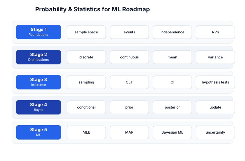
The roadmap moves from foundations (Stage 1), through distributions (Stage 2), statistical inference (Stage 3), Bayes’ theorem (Stage 4), and the ML applications (Stage 5). The Linear Algebra tutorial is the companion piece — the two together are the math of ML.

---

Stage 1 — Foundations

Sample space, events, probability

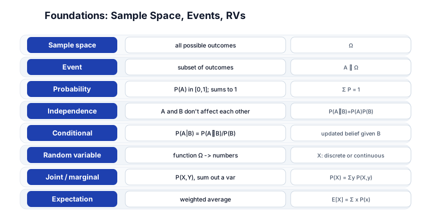
• Sample space (Ω) — the set of all possible outcomes. Rolling a die: Ω = {1, 2, 3, 4, 5, 6}.
• Event (A) — a subset of outcomes. “Roll even”: A = {2, 4, 6}.
• Probability (P) — a function from events to [0, 1], where P(Ω) = 1 and probabilities of disjoint events add: P(A ∪ B) = P(A) + P(B) if A ∩ B = ∅.

Independence and conditional probability

• Independence — A and B are independent if knowing one doesn’t change the other: P(A ∩ B) = P(A) · P(B).
• Conditional probability — P(A | B) = P(A ∩ B) / P(B) — the probability of A given that B happened. This is the foundation of Bayes’ theorem (Stage 4).

Random variables

A random variable (RV) is a function from outcomes to numbers: X: Ω → ℝ. “The number on the die” is a random variable. RVs are discrete (countable values, like dice) or continuous (real values, like height).

Expectation, variance

import numpy as np
# Discrete: E[X] = Σ x · P(x)
x = np.array([1, 2, 3, 4, 5, 6])
p = np.array([1/6]*6)
ex = np.sum(x * p)            # 3.5 — the expected value of a fair die
var = np.sum((x - ex)**2 * p) # 2.917 — the variance

• Expectation E[X] — the long-run average: E[X] = Σ x · P(x) (discrete) or ∫ x · f(x) dx (continuous).
• Variance Var(X) — E[(X - E[X])²], how spread out the distribution is. Standard deviation σ = √Var(X).

Pitfall: “Expected value” is not the value you expect to see — a fair die never shows 3.5. It’s the long-run average over many trials. Confusing the expectation with a typical outcome leads to bad intuition (the lottery has a high expected payout per winner, but you’ll almost certainly lose).

---

Stage 2 — Distributions

Discrete distributions

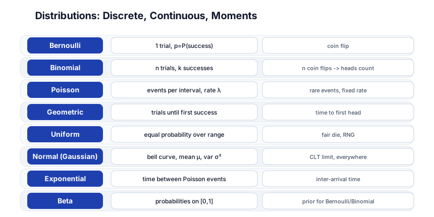
Distribution	What it models	Parameters
Bernoulli	one trial, success/failure	p = P(success)
Binomial	n trials, count of successes	n, p
Poisson	events per interval (rare events, fixed rate)	λ (rate)
Geometric	trials until first success	p
Uniform (discrete)	equal probability over a set	the set

from scipy import stats
stats.binom.pmf(k=3, n=10, p=0.5)  # P(3 heads in 10 flips) = 0.117
stats.poisson.pmf(k=2, mu=3)       # P(2 events, rate 3) = 0.224

Continuous distributions

Distribution	What it models	Parameters
Normal (Gaussian)	the bell curve; everything, by CLT	μ (mean), σ² (variance)
Uniform (continuous)	equal density over an interval	[a, b]
Exponential	time between Poisson events	λ (rate)
Beta	a probability on [0,1]	α, β

The Normal distribution — the most important

stats.norm.pdf(x=0, loc=0, scale=1)    # PDF at 0 = 0.399 (peak)
stats.norm.cdf(x=0, loc=0, scale=1)    # CDF at 0 = 0.5 (half below)
# 68% within 1σ, 95% within 2σ, 99.7% within 3σ (the 68-95-99.7 rule)

The Normal distribution is everywhere because of the Central Limit Theorem (Stage 3) — sample means are approximately Normal regardless of the population. It’s parameterized by mean μ and variance σ², and the PDF is the bell curve f(x) = (1/(σ√2π)) · e^(-(x-μ)²/(2σ²)).

PMF vs PDF vs CDF

• PMF (probability mass function) — for discrete RVs: P(X = x).
• PDF (probability density function) — for continuous RVs: f(x), where P(a ≤ X ≤ b) = ∫ₐᵇ f(x) dx. Note: P(X = x) = 0 for a continuous RV (a single point has zero probability).
• CDF (cumulative distribution function) — F(x) = P(X ≤ x), works for both.

Pitfall: For a continuous RV, P(X = 5) = 0 — you can’t ask “the probability of exactly 5.” You ask “the probability of being between 4.9 and 5.1” (an integral over the PDF). The PDF f(5) is a density, not a probability — it can be greater than 1 (e.g. a narrow peak).

---

Stage 3 — Statistical Inference

Sampling distributions and the Central Limit Theorem

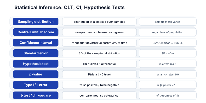
The Central Limit Theorem (CLT): the sample mean X̄ of n independent draws is approximately Normal as n grows, regardless of the population distribution. The mean of the sample mean is μ (the population mean); its standard deviation (the standard error) is σ/√n.

# CLT in action: sample means of 1000 dice rolls are roughly Normal
samples = np.random.randint(1, 7, size=(10000, 30)).mean(axis=1)
# samples is approximately Normal(3.5, 2.917/√30 = 0.31)

This is why the Normal distribution is everywhere — sample means, proportions, and many statistics converge to Normal. It’s the foundation of confidence intervals and hypothesis tests.

Confidence intervals

A 95% confidence interval is a range that, over many samples, contains the true parameter 95% of the time. For a mean with known σ:

mean = data.mean()
se = data.std() / np.sqrt(len(data))   # standard error
ci = (mean - 1.96 * se, mean + 1.96 * se)   # 95% CI (1.96 = z for 95%)

Pitfall: A 95% CI is not “there’s a 95% chance the true value is in this interval” (the true value is fixed; the interval either contains it or not). It’s “if I repeated this procedure 100 times, ~95 of the intervals would contain the true value.” The randomness is in the interval, not the parameter (frequentist view).

Hypothesis testing

• H₀ (null) — the default (no effect, no difference).
• H₁ (alternative) — what we’re testing for (there is an effect).
• p-value — P(data as extreme as observed | H₀ true). Small p → reject H₀.
• Significance level α — the threshold (commonly 0.05); reject if p < α.

Type I and Type II errors

	H₀ true	H₀ false
Reject H₀	Type I error (false positive), probability α	correct (true positive)
Fail to reject	correct (true negative)	Type II error (false negative), probability β

Power = 1 - β — the probability of detecting a real effect. Underpowered studies fail to detect real effects; this is why sample size matters.

Pitfall: p-hacking — running many tests and reporting only the significant ones inflates the false-positive rate. With 20 independent tests at α=0.05, you’d expect ~1 false positive by chance. Correct with multiple-comparison correction (Bonferroni, FDR).

---

Stage 4 — Bayes’ Theorem

The rule that updates beliefs

Bayes’ theorem updates a belief given new evidence:

P(H | D) = P(D | H) · P(H) / P(D)

• P(H) — prior: belief about hypothesis H before seeing data.

• **P(D

  H)** — likelihood: how likely the data is if H is true.

• **P(H

  D)** — posterior: updated belief after seeing the data.

• P(D) — evidence: normalizing constant (often ignored in comparison).

# Medical test example: disease rate 1%, test 99% sensitive + 95% specific
prior = 0.01
likelihood = 0.99          # P(+ | disease)
false_positive = 0.05      # P(+ | no disease)
evidence = likelihood * prior + false_positive * (1 - prior)
posterior = likelihood * prior / evidence   # P(disease | +) = 0.167

You test positive on a 99%-sensitive test for a 1%-prevalence disease — your probability of actually having it is only 16.7%, because the prior (1%) dominates. This is why base rates matter and why screening tests for rare diseases have high false-positive rates.

Bayesian updating

Bayesian inference is iterative: today’s posterior is tomorrow’s prior. Each new piece of evidence updates the belief. This is the formal version of “learning from data” — and it’s exactly what ML training does (Stage 5).

---

Stage 5 — ML: MLE, MAP, Bayesian Inference

MLE — Maximum Likelihood Estimation

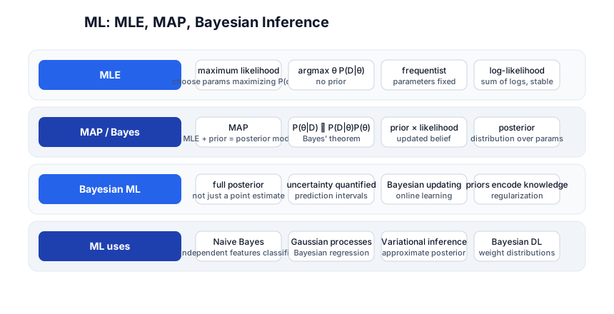
MLE finds the parameters that maximize the probability of the observed data:

θ_MLE = argmax_θ P(D | θ) = argmax_θ Π P(xᵢ | θ)

# MLE for a Normal distribution: μ = sample mean, σ² = sample variance
mu_mle = data.mean()
sigma2_mle = data.var()

MLE is frequentist: the parameters are fixed (unknown) constants, and we find the ones that best explain the data. No prior. Linear regression’s least-squares solution is the MLE under Gaussian noise. Logistic regression’s cross-entropy loss is the negative log-likelihood of a Bernoulli. Most ML training is MLE (or a regularized version of it).

MAP — Maximum A Posteriori

MAP adds a prior to MLE — it finds the parameters that maximize the posterior:

θ_MAP = argmax_θ P(D | θ) · P(θ) = argmax_θ [likelihood × prior]

MAP is MLE + regularization: a Gaussian prior on the weights is L2 regularization (ridge); a Laplace prior is L1 regularization (LASSO). “Regularization = a prior” is the bridge between frequentist and Bayesian ML.

Bayesian inference — the full posterior

Bayesian inference goes further than MAP — instead of a single best parameter, it computes the full posterior distribution P(θ | D). This gives you uncertainty estimates: not just “the best weight is 0.7” but “the weight is probably between 0.5 and 0.9.” This is the core advantage of Bayesian ML — calibrated uncertainty, crucial for safety-critical applications (medicine, autonomous driving) where “I’m 60% confident” matters more than “my best guess is X”.

Naive Bayes

Naive Bayes is a classifier based on Bayes’ theorem with a “naive” assumption that features are conditionally independent given the class:

P(class | features) ∝ P(class) · Π P(featureᵢ | class)

It’s simple, fast, and works surprisingly well for text classification (spam, sentiment) — even though the independence assumption is almost always violated, the ranking of classes is robust.

Where probability shows up in ML

ML concept	Probability foundation
Cross-entropy loss	negative log-likelihood (MLE)
L2 / L1 regularization	Gaussian / Laplace prior (MAP)
Softmax	turns logits into a categorical distribution
Naive Bayes	Bayes’ theorem + conditional independence
Gaussian mixture models	mixture of Normal distributions
Gaussian processes	distribution over functions (Bayesian regression)
Variational inference	approximate a posterior with a simpler distribution
Bayesian neural networks	distributions over weights, not point estimates

Pitfall: A neural network’s softmax output is not a calibrated probability — a 0.9 doesn’t mean “90% likely to be correct.” It’s a score that ranks classes well but is systematically overconfident. Temperature scaling or Bayesian methods calibrate it; this matters when you’re using the probability to make a decision (medical diagnosis, fraud).

---

Quick-Start Checklist

1. Install scipy + numpy — pip install scipy numpy.
2. Compute expectations + variance — np.sum(x * p), np.sum((x - ex)**2 * p).
3. Plot distributions — scipy.stats.norm.pdf, binom.pmf, poisson.pmf.
4. Simulate the CLT — sample means of 30 dice rolls → histogram → roughly Normal.
5. Compute a 95% CI — mean ± 1.96 · (std/√n).
6. Run a hypothesis test — scipy.stats.ttest_ind(group1, group2) → p-value.
7. Apply Bayes’ theorem — posterior = likelihood × prior / evidence.
8. Compute MLE for a Normal — μ = data.mean(), σ² = data.var().
9. See MAP = regularization — fit ridge regression; it’s MLE + Gaussian prior.
10. Train Naive Bayes — sklearn.naive_bayes.GaussianNB on a dataset.

Common Pitfalls

• Expected value ≠ typical outcome — a fair die shows 3.5 in expectation but never 3.5 in reality.
• PDF is a density, not a probability — f(x) can be > 1; P(X = x) = 0 for continuous RVs.
• Misreading a confidence interval — it’s about the procedure, not “95% chance the value is in here.”
• p-hacking — many tests + cherry-picking inflates false positives; correct for multiple comparisons.
• Ignoring base rates (Bayes) — a 99%-sensitive test for a 1%-prevalence disease is mostly false positives.
• Confusing MLE and MAP — MLE has no prior; MAP = MLE + prior = MLE + regularization.
• Treating softmax as calibrated probability — neural nets are overconfident; calibrate for decisions.
• Underpowered tests — small n means high Type II error (missed real effects).

Further Reading

• Introduction to Probability by Grinstead & Snell — free textbook
• Bayesian Data Analysis by Gelman et al — the Bayesian bible
• Pattern Recognition and Machine Learning by Bishop — ML + probability
• Seeing Theory — interactive visual probability
• StatQuest — friendly statistics videos

Related guides

Probability + statistics is the math of ML — these PyShine tutorials connect to it:

• Learn Linear Algebra for ML in One Post — the other half of ML math; vectors + matrices + the data.
• Learn Machine Learning in One Post — every ML algorithm is probability applied.
• Learn Deep Learning in One Post — cross-entropy = log-likelihood; softmax = categorical distribution.
• Learn Python in One Post — numpy + scipy are the Python stats libraries.
• Learn Data Structures and Algorithms in One Post — randomized algorithms + probability of hash collisions.

---

Probability and statistics is the language ML is written in: every model is a distribution, every loss is a likelihood, every regularization is a prior, and every evaluation is an inference. The five stages here — foundations, distributions, inference, Bayes, ML applications — cover everything from a fair die to a Bayesian neural network with calibrated uncertainty. The two insights that pay off forever: the CLT makes the Normal distribution universal (sample means are Normal regardless of the population), and MAP = MLE + prior = regularization (the bridge between frequentist and Bayesian ML, and why L2 regularization “works”). Roll 1000 dice in Python, plot the sample-mean histogram, and watch the bell curve appear — once you’ve seen the CLT, the rest of statistics clicks into place.

Enjoyed this post? Never miss out on future posts by following us