LLM Prompt vs Decode: Understanding the Two Phases of LLM Inference

When you send a request to a large language model – whether through ChatGPT, a local Ollama instance, or a production API – the model does not process your input and generate output in a single uniform step. Instead, every LLM inference request is split into two fundamentally different computational phases: prompt processing (also called prefill) and decoding (also called autoregressive generation).

Understanding the difference between these two phases is essential for anyone working with LLMs – from engineers optimizing inference servers to developers choosing sampling parameters. The two phases have different computational bottlenecks, different memory access patterns, and different optimization strategies. Confusing them leads to poor performance tuning, wrong hardware choices, and misunderstood latency budgets.

The Core Difference in One Sentence

Prompt (prefill) processes all input tokens at once in a single parallel forward pass; decode generates output tokens one at a time, each requiring a separate forward pass that depends on the previous token.

Phase 1: Prompt / Prefill

Understanding the Architecture

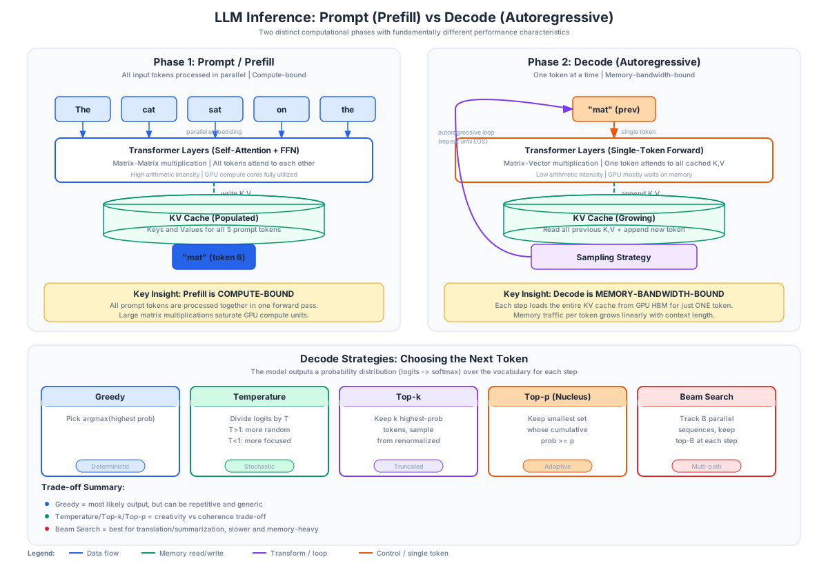
The diagram above illustrates the complete LLM inference pipeline, split into two phases with fundamentally different computational characteristics. Let us break down each component in detail.

Phase 1: Prompt / Prefill (Left Side)

The prefill phase begins when the user’s input prompt arrives at the model. Every token in the prompt – whether it is 10 tokens or 10,000 tokens – is processed simultaneously in a single forward pass through the transformer layers. This is the key property that makes prefill qualitatively different from decoding: all tokens are embedded and attended to each other in parallel.

Token Embedding Layer The input tokens (“The”, “cat”, “sat”, “on”, “the”) are first converted into dense vector representations through an embedding lookup. This step is essentially free in computational terms – it is a simple table lookup that maps each token ID to a high-dimensional vector (typically 4096 to 12288 dimensions for modern LLMs). All five tokens are embedded simultaneously with no sequential dependency.

Transformer Layers (Parallel Computation) Once embedded, all token vectors pass through the transformer layers together. At each layer, the self-attention mechanism allows every token to attend to every other token in the prompt. This means the computation is a dense matrix-matrix multiplication: the query matrix (all tokens) is multiplied by the key matrix (all tokens), producing an attention score matrix of size N x N where N is the prompt length. This is where the GPU’s tensor cores shine – large matrix multiplications are exactly what GPUs are designed for.

The arithmetic intensity (ratio of FLOPs to bytes transferred from memory) is high during prefill because the matrices are large. The GPU compute cores are fully saturated, making this phase compute-bound. Adding more prompt tokens only marginally increases latency because the GPU can parallelize the work across its thousands of cores.

KV Cache Construction As the prompt tokens pass through each transformer layer, the model computes and stores the key (K) and value (V) tensors for every token at every layer. These K,V pairs are written to the KV cache – a persistent memory buffer that will be reused during the decode phase. For a model like Llama-2 7B with 32 layers, 32 attention heads, and 128-dimensional heads, each token’s KV cache consumes approximately 0.5 MB in FP16 precision. A 4,000-token prompt therefore requires roughly 2 GB of KV cache storage.

Output: First Generated Token After the final transformer layer, the model produces a probability distribution (logits) over its entire vocabulary (typically 32,000 to 128,000 tokens). The highest-probability token (or a sampled token, depending on the decoding strategy) becomes the first output token. This token is also the starting point for the decode phase.

Key Performance Characteristic Prefill latency scales sub-linearly with prompt length because the computation is parallelized. Doubling the prompt length does not double the prefill time – it increases it by a much smaller factor because the GPU has spare compute capacity. The primary metric for prefill performance is Time To First Token (TTFT), which measures how long the user waits before seeing the first word of the response.

Phase 2: Decode / Autoregressive Generation

Phase 2: Decode (Right Side)

Once the first token is generated, the model enters the decode phase. This is where the fundamental asymmetry becomes apparent: instead of processing many tokens in parallel, the model now processes exactly ONE token at a time.

Single-Token Forward Pass The most recently generated token is fed back into the transformer as the input. Unlike prefill where all tokens were processed together, here only a single token’s query vector needs to be computed. However, this single query must still attend to ALL previous tokens’ keys and values stored in the KV cache. This transforms the computation from a matrix-matrix multiplication (prefill) into a matrix-vector multiplication (decode).

KV Cache: Read and Append The decode phase reads the entire KV cache from GPU memory (HBM) for every single token it generates. This is the critical bottleneck: the GPU must load potentially gigabytes of KV cache data from memory just to produce one token. After computing the new token’s K,V values, they are appended to the cache, making it slightly larger for the next step.

The arithmetic intensity is extremely low during decode – the GPU performs a tiny amount of computation (one token’s attention) relative to the massive amount of data it must load from memory. This makes decoding memory-bandwidth-bound: the GPU’s compute cores are mostly idle, waiting for data to arrive from memory.

Autoregressive Loop After each token is generated, the process repeats: the new token becomes the input for the next step, the KV cache grows by one entry, and another forward pass produces the next token. This loop continues until the model generates an end-of-sequence (EOS) token or a maximum length is reached. The sequential nature of this loop means decode latency scales linearly with output length – 100 output tokens require 100 sequential forward passes.

Key Performance Characteristic Decode latency is measured in Time Per Output Token (TPOT). Because each step is memory-bound, the GPU’s peak compute capability (TFLOPS) is largely irrelevant – what matters is memory bandwidth (GB/s). This is why two GPUs with similar FLOPS but different memory bandwidth can have vastly different decode performance. As context length grows, the KV cache grows, and each decode step becomes slower because more data must be loaded from memory.

Why the Distinction Matters

Aspect	Prompt (Prefill)	Decode (Autoregressive)
Tokens per step	All input tokens	1 token
Computation type	Matrix-matrix	Matrix-vector
Bottleneck	Compute (FLOPS)	Memory bandwidth (GB/s)
GPU utilization	High (cores saturated)	Low (memory-bound)
Latency scaling	Sub-linear with input length	Linear with output length
Primary metric	TTFT (Time To First Token)	TPOT (Time Per Output Token)
KV cache	Write (build)	Read + Append (grow)

This distinction has profound implications for LLM serving infrastructure:

1. Batching strategies differ: During prefill, you want large batches to maximize GPU utilization. During decode, batching helps amortize memory loads but each request in the batch adds its own KV cache to the memory pressure.

2. Hardware selection: For prefill-heavy workloads (short prompts, long outputs), you need high memory bandwidth. For decode-heavy workloads, you need large memory capacity to hold many KV caches.

3. Optimization targets: Systems like vLLM optimize decode through PagedAttention, which reduces KV cache memory waste. Other systems like speculative decoding aim to parallelize the decode phase by guessing multiple future tokens.

Decoding Strategies: Choosing the Next Token

The bottom section of the diagram shows the five most common decoding strategies. After each decode step, the model outputs a probability distribution (logits passed through softmax) over its entire vocabulary. The decoding strategy determines how the next token is selected from this distribution.

1. Greedy Decoding The simplest strategy: always pick the token with the highest probability (argmax). This is deterministic – the same prompt always produces the same output. While fast and predictable, greedy decoding tends to produce repetitive, generic text. It is suitable for factual tasks like translation or code generation where consistency matters more than creativity.

2. Temperature Sampling Before applying softmax, the logits are divided by a temperature value T. When T > 1, the distribution becomes flatter, making lower-probability tokens more likely – this increases randomness and creativity. When T < 1, the distribution becomes sharper, concentrating probability on the top tokens – this makes output more focused and deterministic. Temperature = 0 is equivalent to greedy decoding.

3. Top-k Sampling Only the k highest-probability tokens are kept; the rest are set to zero probability. The remaining k tokens are renormalized and sampled from. This prevents extremely unlikely tokens from being selected while still allowing controlled randomness. A common value is k = 40, which provides a good balance between diversity and coherence.

4. Top-p (Nucleus) Sampling Instead of fixing the number of candidate tokens (like top-k), nucleus sampling keeps the smallest set of tokens whose cumulative probability exceeds a threshold p (typically 0.9 or 0.95). This is adaptive: when the model is confident (one token dominates), only a few candidates are considered. When the model is uncertain (many tokens have similar probability), more candidates are included. Nucleus sampling generally produces the most natural-sounding text.

5. Beam Search Instead of maintaining a single sequence, beam search tracks B parallel sequences (beams) simultaneously. At each step, it expands all beams and keeps the top-B sequences by cumulative log probability. This explores multiple paths and can find higher-quality outputs than single-sequence methods. However, beam search is computationally expensive (B times the memory and compute) and is best suited for tasks like machine translation or summarization where there is a clear quality metric. It is less useful for open-ended text generation where diversity is valued.

Practical Implications for Developers

Choosing a decoding strategy depends on your use case:

• Code generation / factual Q&A: Use greedy or low temperature (T = 0.1-0.3) for deterministic, accurate outputs
• Creative writing / brainstorming: Use temperature (T = 0.7-0.9) or top-p (p = 0.9) for diverse, creative outputs
• Translation / summarization: Use beam search (B = 4-8) for the highest quality structured output
• Chatbots / conversational AI: Use top-p (p = 0.9) with moderate temperature for natural, varied responses

Optimizing inference latency requires understanding which phase dominates:

• If your workload has long prompts and short outputs (e.g., document Q&A), prefill dominates. Optimize by using a faster GPU or reducing prompt length.
• If your workload has short prompts and long outputs (e.g., creative writing), decode dominates. Optimize by using GPUs with higher memory bandwidth or techniques like speculative decoding.

KV cache memory is often the hidden bottleneck. For a 7B parameter model serving a 4,000-token context, each concurrent request requires approximately 2 GB of KV cache. On a 40 GB GPU, this limits you to roughly 15-20 concurrent requests before running out of memory – even though the model weights only occupy 14 GB. This is why systems like vLLM with PagedAttention are critical for production deployments: they reduce KV cache memory waste from 60-80% down to under 4%, dramatically increasing throughput.

Related Concepts

• Speculative decoding: Uses a smaller “draft” model to guess multiple tokens, which the larger model verifies in a single forward pass – partially parallelizing the decode phase
• Flash Attention: Optimizes the attention computation by reducing memory reads/writes, benefiting both prefill and decode
• KV cache quantization: Reduces KV cache memory by storing keys and values in lower precision (e.g., INT8 instead of FP16), trading slight quality loss for 2x memory savings
• Continuous batching: Dynamically adds and removes requests from a batch during decode, maximizing GPU utilization without waiting for all requests to finish

Further Reading

• Attention Is All You Need (Vaswani et al., 2017) – The original Transformer paper that introduced self-attention
• Efficient Memory Management for Large Language Model Serving with PagedAttention (Kwon et al., 2023) – The vLLM paper that revolutionized KV cache management
• Hugging Face KV Cache Documentation – Practical guide to KV cache strategies in the Transformers library

Related Posts

• AI Coding FAQ: 20 Most Asked Questions
• Learn System Design in One Post
• FreeLLMAPI: OpenAI-Compatible Proxy Stacking 16 Free LLM Providers

Conclusion

The distinction between prompt (prefill) and decode (autoregressive) is not just an academic curiosity – it is the single most important factor in understanding LLM inference performance. Prefill is compute-bound and parallelizable; decode is memory-bandwidth-bound and inherently sequential. The decoding strategy you choose (greedy, temperature, top-k, top-p, or beam search) determines the quality and character of the output, while the phase distinction determines which hardware and system optimizations will be effective.

By understanding these two phases, you can make informed decisions about hardware selection, batching strategies, memory management, and decoding parameters – whether you are running a single model locally or serving millions of requests per day in production.

Enjoyed this post? Never miss out on future posts by following us