Learn Elasticsearch and OpenSearch in a Single Post: Complete Tutorial From Inverted Indexes to Sharding and Query DSL

Elasticsearch is a distributed search and analytics engine — it stores JSON documents, builds an inverted index for sub-second full-text search, and scales horizontally across a cluster of nodes. It powers site search, log analytics (the ELK stack), and — increasingly — vector search for AI applications. OpenSearch is the Apache-2.0 fork (maintained by AWS) with the same API. This single post teaches the whole engine in five stages, with hand-drawn diagrams and runnable queries.

Learning Roadmap

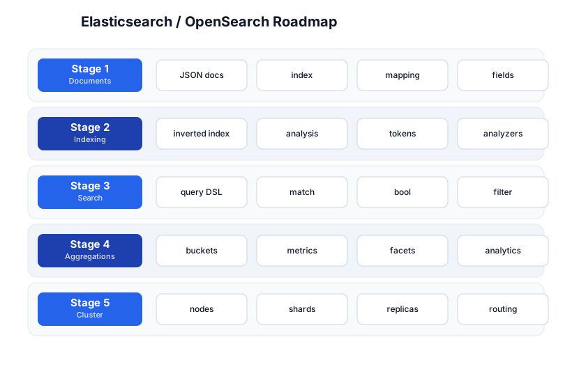
The roadmap moves from the data model (Stage 1), through how it indexes (Stage 2), how you query (Stage 3), analytics (Stage 4), and how it scales (Stage 5).

---

Stage 1 — Documents, Index, Mapping

The data model

Elasticsearch stores documents (JSON objects) in an index (a collection of documents, like a table). Each document has a _id and a set of fields. A mapping defines the schema — the type of each field (text, keyword, integer, date, boolean, etc.).

// Index a document
PUT /products/_doc/1
{
  "name": "Wireless Mouse",
  "category": "electronics",
  "price": 29.99,
  "in_stock": true,
  "tags": ["wireless", "ergonomic"],
  "created": "2026-07-20"
}

Mapping: text vs keyword

The most important distinction in Elasticsearch:

• text — analyzed (tokenized) for full-text search. "Wireless Mouse" → tokens ["wireless", "mouse"]. Used for match queries.
• keyword — exact value, not analyzed. Used for term queries, sorting, and aggregations. "electronics" stays "electronics".

PUT /products
{
  "mappings": {
    "properties": {
      "name":     { "type": "text" },
      "category": { "type": "keyword" },
      "price":    { "type": "float" },
      "in_stock": { "type": "boolean" },
      "created":  { "type": "date" }
    }
  }
}

Often you want both: "category": { "type": "text", "fields": { "raw": { "type": "keyword" } } } — index it as text for search AND as keyword (category.raw) for aggregations/sorting.

Pitfall: Once a field is mapped, you can’t change its type without reindexing. Elasticsearch infers the mapping from the first document you index — so if your first doc has "price": "29.99" (string), it maps price as text, and every subsequent numeric price is rejected. Always define the mapping explicitly before indexing data.

---

Stage 2 — Indexing: The Inverted Index

How search engines are fast

Elasticsearch is fast because it builds an inverted index — a data structure that maps each term to the list of documents that contain it. It’s the same idea as a book’s index: to find “fox”, you look up “fox” and get the pages (documents) that mention it.

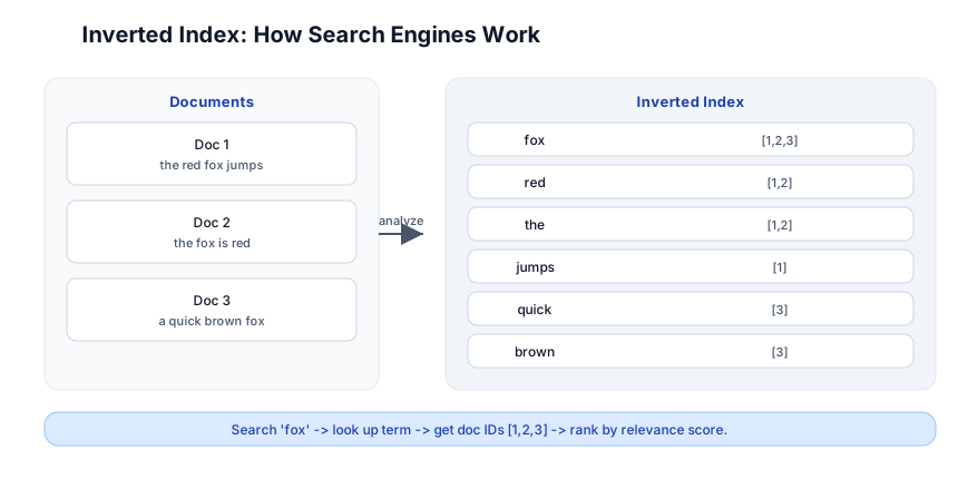
Documents:
  Doc 1: "the red fox jumps"
  Doc 2: "the fox is red"
  Doc 3: "a quick brown fox"

Inverted Index (after analysis):
  fox    -> [1, 2, 3]
  red    -> [1, 2]
  the    -> [1, 2]
  jumps  -> [1]
  quick  -> [3]
  brown  -> [3]

To search for "fox", Elasticsearch looks up fox in the index → [1, 2, 3] → ranks by relevance. It never scans the documents; it looks up a term and gets the answer in O(1).

Analysis: text → tokens

When you index a text field, an analyzer processes it:

1. Character filters — e.g. strip HTML tags.
2. Tokenizer — split text into tokens (words). The standard tokenizer splits on whitespace + punctuation.
3. Token filters — lowercase, stemming (running → run), stop words (the, a), synonyms.

"Wireless Mouse Ergonomic Design"
  -> tokenizer -> ["Wireless", "Mouse", "Ergonomic", "Design"]
  -> lowercase -> ["wireless", "mouse", "ergonomic", "design"]
  -> stemmer   -> ["wireless", "mous", "ergonom", "design"]   (Porter stemmer)
  -> indexed

The same analysis happens to the query — so searching "mice" matches "mouse" if the stemmer maps both to mous.

Choosing an analyzer

Analyzer	What it does
standard (default)	grammar-based tokenizer, lowercase
simple	lowercase + split on non-letters
whitespace	split on whitespace only (keeps case)
english	standard + English stop words + stemming
keyword	no analysis (the whole field is one token)

"mappings": {
  "properties": {
    "description": { "type": "text", "analyzer": "english" }
  }
}

Pitfall: The analyzer applies at index time AND query time — but they must match. If you index with the english analyzer (stemming) and query with standard (no stemming), "mice" won’t match "mouse". Use the search_analyzer field to control query-time analysis separately if needed.

---

Stage 3 — Search: Query DSL

The Query DSL

Elasticsearch uses a JSON Query DSL to express searches. The two main categories:

• Full-text queries (match, match_phrase, multi_match) — analyzed, scored by relevance. Used on text fields.
• Term-level queries (term, terms, range, exists) — not analyzed, exact match. Used on keyword, numeric, date fields.

GET /products/_search
{
  "query": {
    "match": {
      "name": "wireless mouse"
    }
  }
}

match analyzes "wireless mouse" → ["wireless", "mouse"], looks up both terms, and returns documents containing either, ranked by BM25 (a TF-IDF variant) relevance score.

The bool query — combining clauses

GET /products/_search
{
  "query": {
    "bool": {
      "must":     [{ "match": { "name": "wireless mouse" } }],
      "filter":   [{ "term":  { "category": "electronics" } },
                    { "range": { "price": { "lte": 50 } } }],
      "should":   [{ "match": { "tags": "ergonomic" } }],
      "must_not": [{ "term":  { "in_stock": false } }]
    }
  }
}

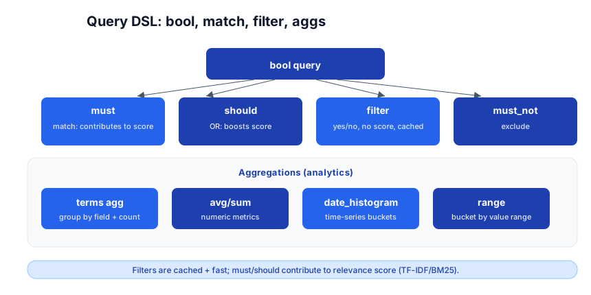
Clause	Role
must	must match AND contributes to score (AND)
filter	must match, but no score — just yes/no. Cached + fast.
should	optional, boosts score if it matches (OR)
must_not	must not match (NOT)

Pitfall: Put exact-match conditions (category, price range, status) in filter, not must. Filters don’t compute a score and are cached — often 10x faster than must. Use must only for relevance-ranked full-text matches.

Scoring: BM25

The relevance score is computed by BM25 (Okapi BM25), which considers:

• Term frequency in the document (more occurrences = more relevant, but saturating).
• Inverse document frequency (rare terms are more valuable than common ones).
• Document length (shorter docs that match are more relevant than long ones).

The _score field in results is the BM25 score. You can boost fields ("name^3": "wireless") to weight them higher.

---

Stage 4 — Aggregations

Analytics on top of search

Aggregations compute analytics over your documents — group, count, average, etc. They’re the SQL GROUP BY + SUM/AVG of Elasticsearch, and they run on the same query (in one round trip).

GET /products/_search
{
  "size": 0,
  "query": { "match": { "category": "electronics" } },
  "aggs": {
    "by_category": {
      "terms": { "field": "category.keyword", "size": 10 },
      "aggs": {
        "avg_price": { "avg": { "field": "price" } },
        "price_range": {
          "range": { "field": "price", "ranges": [{ "to": 25 }, { "from": 25, "to": 100 }, { "from": 100 }] }
        }
      }
    }
  }
}

Two kinds:

• Bucket aggregations — group documents into buckets (terms, range, date_histogram, histogram). Like GROUP BY.
• Metric aggregations — compute a value per bucket (avg, sum, max, min, cardinality, percentiles). Like SUM/AVG.

You can nest them: bucket by category → per category, avg price + a price-range histogram. "size": 0 means “don’t return documents, just the aggregations” (you usually don’t want the hits when you’re computing analytics).

Time series: date_histogram

"aggs": {
  "orders_over_time": {
    "date_histogram": { "field": "created", "calendar_interval": "day" },
    "aggs": { "daily_revenue": { "sum": { "field": "price" } } }
  }
}

This is the foundation of the ELK stack’s log dashboards — bucket logs by day/hour, count per bucket, plot in Kibana.

Pitfall: Aggregations run on keyword/numeric/date fields, not text — you can’t aggregate a text field (it’s tokenized into multiple terms). Use the .keyword sub-field or map the field as keyword.

---

Stage 5 — The Cluster

Nodes, shards, replicas

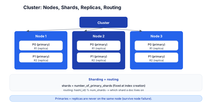
An Elasticsearch cluster is a set of nodes (servers). An index is split into shards — each shard is an independent Lucene index (a piece of the data). Each shard has primaries and replicas (copies for high availability + throughput).

• Primary shards — the original. The number is fixed at index creation (e.g. 3).
• Replica shards — copies of a primary. Can be changed later. Provide redundancy (survive node failure) and read throughput.
• A primary and its replica are never on the same node (so a node failure doesn’t lose data).

Routing: which shard has my document?

shard = hash(_id) % number_of_primary_shards

A document with _id 42 always lives on the same shard (deterministic). This is why the primary shard count is fixed — changing it would re-route every document to a different shard, breaking the index. To “change” the shard count, you reindex into a new index.

Node roles

Role	Function
master-eligible	cluster management (metadata, shard allocation)
data	holds shards, does indexing + search
coordinating	receives requests, fans out to shards, gathers results
ingest	pre-processes documents (pipeline) before indexing

Every node can play multiple roles; in small clusters one node does everything. In large clusters, you separate dedicated masters (3, for stability) from data nodes.

Scale and capacity

• More shards → more parallelism (one query per shard), but more overhead (each shard is a Lucene index). Aim for ~10-50 GB per shard.
• More replicas → more read throughput + availability, but more storage + indexing overhead (every write goes to all replicas).
• Hot-warm architecture — put recent/hot data on fast SSD nodes, older data on cheap storage nodes (via index lifecycle management).

Pitfall: Over-sharding — creating thousands of tiny shards — is the #1 Elasticsearch scaling problem. Each shard uses memory (heap for the segment + filter cache) and cluster state. Don’t create an index with 100 shards if it’ll hold 1 GB of data; 1-3 shards is plenty. Size shards to 10-50 GB, and use the rollover + ILM pattern for time-series data (one index per day/week, sized to the sweet spot).

---

The Ecosystem

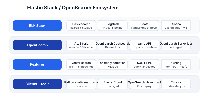
The ELK Stack

• Elasticsearch — search + storage.
• Logstash — ingest pipeline (read from many sources, transform, write to ES).
• Kibana — dashboards, visualization, management UI.
• Beats — lightweight agents (Filebeat for logs, Metricbeat for metrics) that ship data to Logstash or directly to ES.

OpenSearch (the AWS fork)

Elasticsearch changed its license in 2021; AWS forked it as OpenSearch (Apache 2.0). It’s API-compatible (drop-in for most uses), with OpenSearch Dashboards (the Kibana fork). AWS’s managed offering is Amazon OpenSearch Service (and OpenSearch Serverless). For new projects that want a permissive license, OpenSearch is the choice.

Vector search

Both Elasticsearch (with the dense_vector field type + kNN search) and OpenSearch support vector search — storing ML embeddings and finding the nearest neighbors by cosine distance. This powers semantic search, recommendation, and RAG (retrieval-augmented generation) for LLMs. It’s the bridge between the search engine and the ML/embeddings world.

---

Quick-Start Checklist

1. Run Elasticsearch — docker run -p 9200:9200 -e discovery.type=single-node docker.elastic.co/elasticsearch/elasticsearch:8.x (or OpenSearch).
2. Create an index with a mapping — define text vs keyword explicitly before indexing.
3. Index a few documents — PUT /products/_doc/1.
4. Run a match query — see the _score and ranked results.
5. Build a bool query with must (full-text) + filter (exact).
6. Run an aggregation — terms agg on category + avg on price.
7. Add a replica — update the index to have 1 replica; see it allocated.
8. Set up Kibana (or OpenSearch Dashboards) and explore the Discover + Visualize tabs.
9. Try vector search — index dense_vector fields and run a kNN query.
10. Use ILM + rollover for time-series data to avoid over-sharding.

Common Pitfalls

• Implicit mapping from first doc — "price": "29.99" maps price as text forever. Define the mapping first.
• Changing a field type — impossible without reindexing into a new index. Get the mapping right upfront.
• text vs keyword confusion — text for full-text search (analyzed), keyword for exact/sort/agg. Use multi-fields (field.keyword) for both.
• Filters in must — slower than filter; filters are cached and skip scoring. Use filter for exact conditions.
• Aggregating a text field — fails or returns weird results; aggregate the .keyword sub-field.
• Over-sharding — too many tiny shards waste memory + cluster state. Aim for 10-50 GB per shard.
• Fixed primary shard count — can’t change after creation; reindex to a new index to resize.
• No dedicated masters — in large clusters, data nodes doing master work cause instability. Use 3 dedicated masters.
• Unbounded size in queries — GET /_search with no size returns 10 by default but deep pagination via from/size is expensive; use search_after or scroll for large result sets.

Further Reading

• Elasticsearch Docs — the official reference
• Elasticsearch: The Definitive Guide — the canonical book (free online)
• OpenSearch Docs — the fork’s docs
• Elasticsearch in Action by Matthew Lee — practical
• Open Distro / OpenSearch Blog — ecosystem updates

Related guides

Elasticsearch is the search + analytics layer of the data stack — these PyShine tutorials connect to it:

• Learn PostgreSQL in One Post — Postgres has full-text search (tsvector) + pgvector; Elasticsearch is the dedicated search alternative at scale.
• Learn Linear Algebra for ML in One Post — vector search (kNN) is cosine/dot-product similarity on embeddings.
• Learn Machine Learning in One Post — embeddings (Stage 3) power semantic search in Elasticsearch.
• Learn Apache Kafka in One Post — Kafka + ELK is the classic log pipeline (Kafka ingests, Logstash transforms, ES indexes, Kibana viz).
• Learn Observability in One Post — Loki is the lightweight log alternative; ES/Kibana is the heavyweight one for full-text log search.

---

Elasticsearch’s power is the inverted index — it never scans documents; it looks up a term and gets the answer. The five stages here — documents, indexing, search, aggregations, cluster — cover everything from a single-node index to a sharded, replicated, aggregation-driven analytics cluster with vector search. The two habits that pay off: define your mapping before indexing (implicit mapping is a footgun), and use filter for exact conditions and must for relevance (filters are cached and fast; must computes a score you may not need). Run Elasticsearch in Docker, index 5 documents, run a bool query with a match + filter, and watch the _score rank the results — once you’ve seen the inverted index at work, the model clicks.

Enjoyed this post? Never miss out on future posts by following us